AE 03: Bootstrap confidence intervals

Bikeshare

Author

Driver: ____, Reporter: _____, Gopher: _____

Published

September 6, 2024

Important

Open RStudio and create a subfolder in your AE folder called “AE-03”
Go to the course Canvas page and locate your AE 03 assignment to get started.
Upload the ae-03.qmd and dcbikeshare.csv files into the folder you just created.

The .qmd and .pdf files uploaded to Canvas no later than Monday, September 9 at 11:59pm.

library(tidyverse)
library(ggformula)
library(broom)
library(infer)
library(openintro)
library(kableExtra)

Data

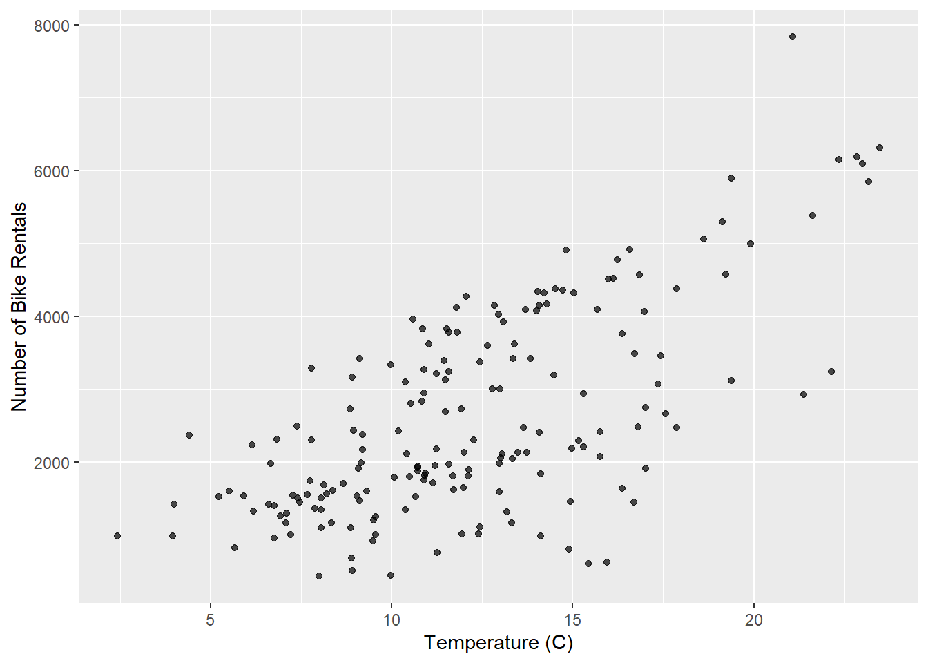
Our dataset contains daily rentals from the Capital Bikeshare in Washington, DC in 2011 and 2012 filtered to only contain the winter months. It was obtained from the dcbikeshare data set in the dsbox R package.

We will focus on the following variables in the analysis:

count: total bike rentals
temp_orig: Temperature in degrees Celsius

winter <- read_csv("../ae/data/dcbikeshare.csv") |>
  mutate(season = case_when(
    season == 1 ~ "winter",
    season == 2 ~ "spring",
    season == 3 ~ "summer",
    season == 4 ~ "fall"
  ),
  season = factor(season)) |>
  filter(season == "winter")

Rows: 731 Columns: 17
── Column specification ────────────────────────────────────────────────────────
Delimiter: ","
dbl  (16): instant, season, yr, mnth, holiday, weekday, workingday, weathers...
date  (1): dteday

ℹ Use `spec()` to retrieve the full column specification for this data.
ℹ Specify the column types or set `show_col_types = FALSE` to quiet this message.

glimpse(winter)

Rows: 181
Columns: 17
$ instant    <dbl> 1, 2, 3, 4, 5, 6, 7, 8, 9, 10, 11, 12, 13, 14, 15, 16, 17, …
$ dteday     <date> 2011-01-01, 2011-01-02, 2011-01-03, 2011-01-04, 2011-01-05…
$ season     <fct> winter, winter, winter, winter, winter, winter, winter, win…
$ yr         <dbl> 0, 0, 0, 0, 0, 0, 0, 0, 0, 0, 0, 0, 0, 0, 0, 0, 0, 0, 0, 0,…
$ mnth       <dbl> 1, 1, 1, 1, 1, 1, 1, 1, 1, 1, 1, 1, 1, 1, 1, 1, 1, 1, 1, 1,…
$ holiday    <dbl> 0, 0, 0, 0, 0, 0, 0, 0, 0, 0, 0, 0, 0, 0, 0, 0, 1, 0, 0, 0,…
$ weekday    <dbl> 6, 0, 1, 2, 3, 4, 5, 6, 0, 1, 2, 3, 4, 5, 6, 0, 1, 2, 3, 4,…
$ workingday <dbl> 0, 0, 1, 1, 1, 1, 1, 0, 0, 1, 1, 1, 1, 1, 0, 0, 0, 1, 1, 1,…
$ weathersit <dbl> 2, 2, 1, 1, 1, 1, 2, 2, 1, 1, 2, 1, 1, 1, 2, 1, 2, 2, 2, 2,…
$ temp       <dbl> 0.3441670, 0.3634780, 0.1963640, 0.2000000, 0.2269570, 0.20…
$ atemp      <dbl> 0.3636250, 0.3537390, 0.1894050, 0.2121220, 0.2292700, 0.23…
$ hum        <dbl> 0.805833, 0.696087, 0.437273, 0.590435, 0.436957, 0.518261,…
$ windspeed  <dbl> 0.1604460, 0.2485390, 0.2483090, 0.1602960, 0.1869000, 0.08…
$ casual     <dbl> 331, 131, 120, 108, 82, 88, 148, 68, 54, 41, 43, 25, 38, 54…
$ registered <dbl> 654, 670, 1229, 1454, 1518, 1518, 1362, 891, 768, 1280, 122…
$ count      <dbl> 985, 801, 1349, 1562, 1600, 1606, 1510, 959, 822, 1321, 126…
$ temp_orig  <dbl> 14.110847, 14.902598, 8.050924, 8.200000, 9.305237, 8.37826…

Exploratory data analysis

gf_point(count ~ temp_orig, data = winter, alpha = 0.7) |> 
  gf_labs(
    x = "Temperature (C)",
    y = "Number of Bike Rentals",
  )

Model

model_fit <- lm(count ~ temp_orig, data = winter)

tidy(model_fit) |>
  kable(digits = 2)

term	estimate	std.error	statistic	p.value
(Intercept)	-111.04	238.31	-0.47	0.64
temp_orig	222.42	18.46	12.05	0.00

Bootstrap confidence interval

1. Calculate the observed fit (slope)

observed_fit <- winter |>
  specify(count ~ temp_orig) |>
  fit()

observed_fit

# A tibble: 2 × 2
  term      estimate
  <chr>        <dbl>
1 intercept    -111.
2 temp_orig     222.

2. Take n bootstrap samples and fit models to each one.

Fill in the code, then set eval: true .

n = 100
set.seed(212)

boot_fits <- ______ |>
  specify(______) |>
  generate(reps = ____, type = "bootstrap") |>
  fit()

boot_fits

Why do we set a seed before taking the bootstrap samples?
Make a histogram of the bootstrap samples to visualize the bootstrap distribution.
```
# Code for histogram
```

3. Compute the 95% confidence interval as the middle 95% of the bootstrap distribution

Fill in the code, then set eval: true .

get_confidence_interval(
  boot_fits, 
  point_estimate = _____, 
  level = ____,
  type = "percentile"
)

Changing confidence level

Modify the code from Step 3 to create a 90% confidence interval.

# Paste code for 90% confidence interval

Modify the code from Step 3 to create a 99% confidence interval.

# Paste code for 90% confidence interval

Which confidence level produces the most accurate confidence interval (90%, 95%, 99%)? Explain
Which confidence level produces the most precise confidence interval (90%, 95%, 99%)? Explain
If we want to be very certain that we capture the population parameter, should we use a wider or a narrower interval? What drawbacks are associated with using a wider interval?

Important

To submit the AE:

Render the document to produce the PDF file with all of your work from today’s class.
Upload your .qmd file and your .pdf file to Canvas. Note, please unzip the folder you download from the RStudio platform before uploading it.