library(tidyverse)
library(ggformula)
library(mosaic)
library(broom)
library(knitr)
library(openintro)

loan50 <- loan50 |>
mutate(annual_income_k = annual_income / 1000)AE 12: Categorical Predictors
Pee-to-Peer Loans
Important
Packages + data
The data for this AE is is a sample of 10,000 loans made through a peer-to-peer lending club. The data is in the loan50 data frame in the openintro R package.
Variables
annual_income_k: Annual income in $1,000’sverified_income: Whether borrower’s income source and amount have been verified (Not Verified,Source Verified,Verified)
Response: interest_rate: Interest rate for the loan
Analysis goal
- Predict
interest_rateusing the categorical variableverified_incomeas a predictor - Include other quantitative variables and understand how they interact with
verified_income
Exercise 1
Generate side-by-side boxplots of interest_rate vs. verified_income. Does it appear that there is a relationship between the two variables?
Exercise 2
Based on the output of the code below, what do you think would be the best predictions for the interest rate of a borrow with Not Verified, Source Verified, and Verified income, respectively.
favstats(interest_rate ~ verified_income, data = loan50) |>
kable()| verified_income | min | Q1 | median | Q3 | max | mean | sd | n | missing |
|---|---|---|---|---|---|---|---|---|---|
| NA | NA | NA | NA | NA | NaN | NA | 0 | 0 | |
| Not Verified | 5.31 | 7.9600 | 9.44 | 9.9300 | 18.45 | 9.541429 | 2.984269 | 21 | 0 |
| Source Verified | 6.08 | 7.8075 | 10.91 | 16.2875 | 19.42 | 11.765500 | 4.270998 | 20 | 0 |
| Verified | 5.32 | 11.9800 | 14.08 | 21.4500 | 26.30 | 15.853333 | 7.694652 | 9 | 0 |
Exercise 3
Fit a linear model predicting interest_rate from verified_income. What is the reference level for verified_income?
Exercise 4
WITHOUT WRITING ANY CODE except for addition, subtraction, multiplication, and addition, what would the model predict the average interest_rate for each of the three levels of verified_income? How do these answers compare to your answers from Exercise 2?
Exercise 5
The linear model below predicts interest_rate from annual_income_k. Add verified_income as a predictor to this model. Do not include an interaction term. Be prepared to discuss how and why the plot changes when you add in verified_income.
ex5_model <- lm(interest_rate ~ annual_income_k, data = loan50)
ex5_model |>
  tidy() |>
kable()| term | estimate | std.error | statistic | p.value |
|---|---|---|---|---|
| (Intercept) | 12.994265 | 1.2851395 | 10.111171 | 0.0000000 |
| annual_income_k | -0.016561 | 0.0124397 | -1.331308 | 0.1893763 |
plotModel(ex5_model) # nifty function from the mosaic package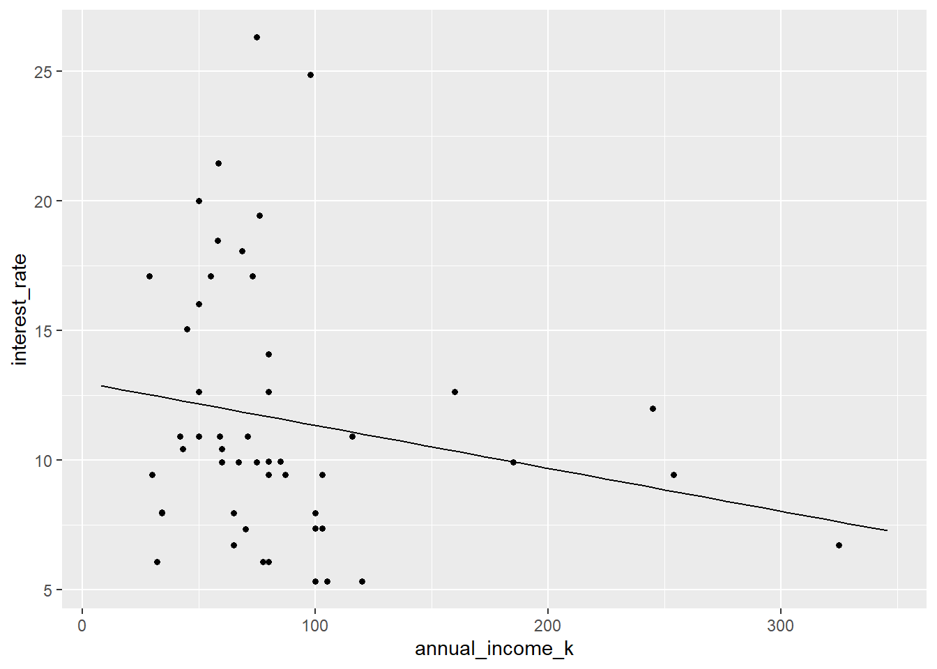
Exercise 6
How do you think the plot above will change if you add in an interaction term between verified_income and interest_rate? AFTER thinking about it, add in an interaction term between verified_income and annual_income_k.
ex6_model <- lm(interest_rate ~ annual_income_k, data = loan50)
ex6_model |>
  tidy() |>
kable()| term | estimate | std.error | statistic | p.value |
|---|---|---|---|---|
| (Intercept) | 12.994265 | 1.2851395 | 10.111171 | 0.0000000 |
| annual_income_k | -0.016561 | 0.0124397 | -1.331308 | 0.1893763 |
plotModel(ex6_model) # nifty function from the mosaic package
Exercise 7
Based on the model above (and the equation on the slides):
- Write the equation of the model to predict interest rate for applicants with Not Verified income.
- Write the equation of the model to predict interest rate for applicants with Verified income.
- Our degrees of freedom will be \(n-p-1\). What is \(p\) in this case? Hint: it isn’t 2.
To submit the AE
Important
- Render the document to produce the PDF with all of your work from today’s class.
- Upload your QMD and PDF files to the Canvas assignment.