SLR: Mathematical models for inference

Prof. Eric Friedlander

Sep 09, 2024

Application exercise

📋 AE 04: Randomization test for the slope

Mathematical models for inference

Topics

• Define mathematical models to conduct inference for the slope

• Use mathematical models to

  • calculate confidence interval for the slope

  • conduct a hypothesis test for the slope

Computational setup

# load packages
library(tidyverse)   # for data wrangling and visualization
library(broom)       # for formatting model output
library(scales)      # for pretty axis labels
library(knitr)       # for pretty tables
library(kableExtra)  # also for pretty tables
library(patchwork)   # arrange plots

# HEB Dataset
heb <- read_csv("data/HEBIncome.csv") |> 
  mutate(Avg_Income_K = Avg_Household_Income/1000)

# set default theme and larger font size for ggplot2
ggplot2::theme_set(ggplot2::theme_bw(base_size = 20))

The regression model, revisited

heb_fit <- lm(Number_Organic ~ Avg_Income_K, data = heb)

tidy(heb_fit) |>
  kable(digits = 2)

term	estimate	std.error	statistic	p.value
(Intercept)	-14.72	9.30	-1.58	0.12
Avg_Income_K	0.96	0.13	7.50	0.00

Inference, revisited

• Earlier we computed a confidence interval and conducted a hypothesis test via simulation:
  • CI: Bootstrap the observed sample to simulate the distribution of the slope
  • HT: Permute the observed sample to simulate the distribution of the slope under the assumption that the null hypothesis is true
• Now we’ll do these based on theoretical results, i.e., by using the Central Limit Theorem to define the distribution of the slope and use features (shape, center, spread) of this distribution to compute bounds of the confidence interval and the p-value for the hypothesis test

Mathematical representation of the model

\[ \begin{aligned} Y &= Model + Error \\ &= f(X) + \epsilon \\ &= \mu_{Y|X} + \epsilon \\ &= \beta_0 + \beta_1 X + \epsilon \end{aligned} \]

where the errors are independent and normally distributed:

• independent: Knowing the error term for one observation doesn’t tell you anything about the error term for another observation
• normally distributed: \(\epsilon \sim N(0, \sigma_\epsilon^2)\)

Mathematical representation, visualized

\[ Y|X \sim N(\beta_0 + \beta_1 X, \sigma_\epsilon^2) \]

Image source: Introduction to the Practice of Statistics (5th ed)

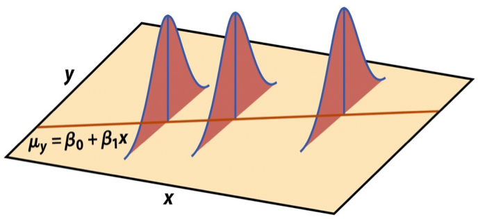
• Mean: \(\beta_0 + \beta_1 X\), the predicted value based on the regression model
• Variance: \(\sigma_\epsilon^2\), constant across the range of \(X\)
  • How do we estimate \(\sigma_\epsilon^2\)?

Regression standard error

Once we fit the model, we can use the residuals to estimate the regression standard error, the average distance between the observed values and the regression line

\[ \hat{\sigma}_\epsilon = \sqrt{\frac{\sum_\limits{i=1}^n(y_i - \hat{y}_i)^2}{n-2}} = \sqrt{\frac{\sum_\limits{i=1}^ne_i^2}{n-2}} \]

1. Why divide by \(n - 2\)?

2. Why do we care about the value of the regression standard error?

Standard error of \(\hat{\beta}_1\)

The standard error of \(\hat{\beta}_1\) quantifies the sampling variability in the estimated slopes

\[ SE_{\hat{\beta}_1} = \hat{\sigma}_\epsilon\sqrt{\frac{1}{(n-1)s_X^2}} \]

term	estimate	std.error	statistic	p.value
(Intercept)	-14.72	9.30	-1.58	0.12
Avg_Income_K	0.96	0.13	7.50	0.00

Mathematical models for inference for \(\beta_1\)

Hypothesis test for the slope

Hypotheses: \(H_0: \beta_1 = 0\) vs. \(H_A: \beta_1 \ne 0\)

Test statistic: Number of standard errors the estimate is away from the null

\[ T = \frac{\text{Estimate - Null Value}}{\text{Standard error}} \\ \]

p-value: Probability of observing a test statistic at least as extreme (in the direction of the alternative hypothesis) from the null value as the one observed

\[ \text{p-value} = P(|T| > |\text{test statistic}|), \]

calculated from a \(t\) distribution with \(n - 2\) degrees of freedom

Hypothesis test: Test statistic

term	estimate	std.error	statistic	p.value
(Intercept)	-14.72	9.30	-1.58	0.12
Avg_Income_K	0.96	0.13	7.50	0.00

\[ T = \frac{\hat{\beta}_1 - 0}{SE_{\hat{\beta}_1}} = \frac{0.96 - 0}{0.13} = 7.38 \]

How should we interpret this test statistic?

Hypothesis test: p-value

term	estimate	std.error	statistic	p.value
(Intercept)	-14.72	9.30	-1.58	0.12
Avg_Income_K	0.96	0.13	7.50	0.00

Hypothesis test: p-value

term	estimate	std.error	statistic	p.value
(Intercept)	-14.72	9.30	-1.58	0.12
Avg_Income_K	0.96	0.13	7.50	0.00

A more exact p-value

2 * pt(q = 7.38, df = 35, lower.tail = FALSE)

[1] 1.243448e-08

Interpret this p-value.

Understanding the p-value

Magnitude of p-value	Interpretation
p-value < 0.01	strong evidence against \(H_0\)
0.01 < p-value < 0.05	moderate evidence against \(H_0\)
0.05 < p-value < 0.1	weak evidence against \(H_0\)
p-value > 0.1	effectively no evidence against \(H_0\)

Important

These are general guidelines. The strength of evidence depends on the context of the problem.

Hypothesis test: Conclusion, in context

term	estimate	std.error	statistic	p.value
(Intercept)	-14.72	9.30	-1.58	0.12
Avg_Income_K	0.96	0.13	7.50	0.00

• The data provide convincing evidence that the population slope \(\beta_1\) is different from 0.
• The data provide convincing evidence of a linear relationship between average household income and the number of organic vegetable options available.

Confidence interval for the slope

\[ \text{Estimate} \pm \text{ (critical value) } \times \text{SE} \]

\[ \hat{\beta}_1 \pm t^* \times SE_{\hat{\beta}_1} \]

where \(t^*\) is calculated from a \(t\) distribution with \(n-2\) degrees of freedom

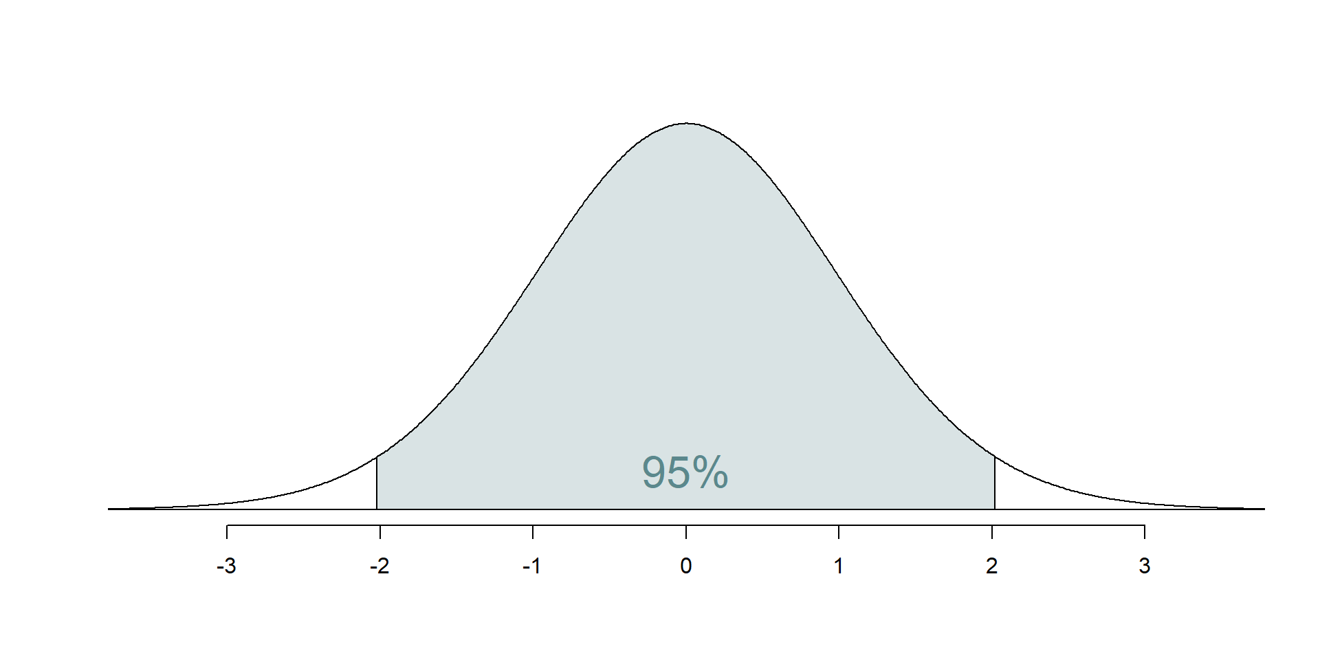
Confidence interval: Critical value

# confidence level: 95%
qt(0.975, df = nrow(heb) - 2)

[1] 2.030108

# confidence level: 90%
qt(0.95, df = nrow(heb) - 2)

[1] 1.689572

# confidence level: 99%
qt(0.995, df = nrow(heb) - 2)

[1] 2.723806

95% CI for the slope: Calculation

term	estimate	std.error	statistic	p.value
(Intercept)	-14.72	9.30	-1.58	0.12
Avg_Income_K	0.96	0.13	7.50	0.00

\[\hat{\beta}_1 = 0.96 \hspace{15mm} t^* = 2.03 \hspace{15mm} SE_{\hat{\beta}_1} = 0.13\]

\[ 0.96 \pm 2.03 \times 0.13 = (0.70, 1.22) \]

95% CI for the slope: Computation

tidy(heb_fit, conf.int = TRUE, conf.level = 0.95) |> 
  kable(digits = 2)

term	estimate	std.error	statistic	p.value	conf.low	conf.high
(Intercept)	-14.72	9.30	-1.58	0.12	-33.59	4.16
Avg_Income_K	0.96	0.13	7.50	0.00	0.70	1.22

Intervals for predictions

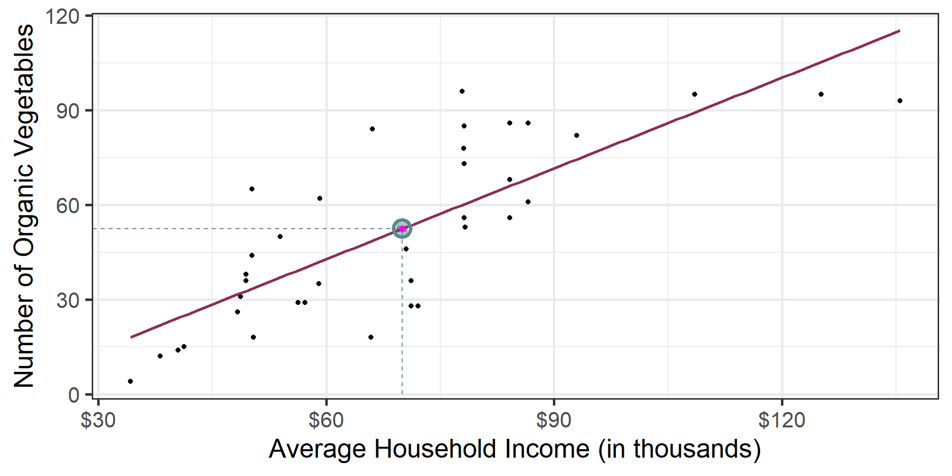
Intervals for predictions

• Question: “What is the predicted number of organic vegetable options in a neighborhood with an average income of $70k?”
• We said reporting a single estimate for the slope is not wise, and we should report a plausible range instead
• Similarly, reporting a single prediction for a new value is not wise, and we should report a plausible range instead

Two types of predictions

1. Prediction for the mean: “What is the average predicted number of organic vegetable options in a neighborhood with an average income of $70k?”

2. Prediction for an individual observation: “What is the predicted number of organic vegetable options at a single HEB in a neighborhood with an average income of $70k?”

Which would you expect to be more variable? The average prediction or the prediction for an individual observation? Based on your answer, how would you expect the widths of plausible ranges for these two predictions to compare?

Uncertainty in predictions

Confidence interval for the mean outcome: \[\large{\hat{y} \pm t_{n-2}^* \times \color{purple}{\mathbf{SE}_{\hat{\boldsymbol{\mu}}}}}\]

Prediction interval for an individual observation: \[\large{\hat{y} \pm t_{n-2}^* \times \color{purple}{\mathbf{SE_{\hat{y}}}}}\]

Standard errors

Standard error of the mean outcome: \[SE_{\hat{\mu}} = \hat{\sigma}_\epsilon\sqrt{\frac{1}{n} + \frac{(x-\bar{x})^2}{\sum\limits_{i=1}^n(x_i - \bar{x})^2}}\]

Standard error of an individual outcome: \[SE_{\hat{y}} = \hat{\sigma}_\epsilon\sqrt{1 + \frac{1}{n} + \frac{(x-\bar{x})^2}{\sum\limits_{i=1}^n(x_i - \bar{x})^2}}\]

Standard errors

Standard error of the mean outcome: \[SE_{\hat{\mu}} = \hat{\sigma}_\epsilon\sqrt{\frac{1}{n} + \frac{(x-\bar{x})^2}{\sum\limits_{i=1}^n(x_i - \bar{x})^2}}\]

Standard error of an individual outcome: \[SE_{\hat{y}} = \hat{\sigma}_\epsilon\sqrt{\mathbf{\color{purple}{\Large{1}}} + \frac{1}{n} + \frac{(x-\bar{x})^2}{\sum\limits_{i=1}^n(x_i - \bar{x})^2}}\]

Confidence interval

The 95% confidence interval for the mean outcome:

new_neighborhood <- tibble(Avg_Income_K = 70)

predict(heb_fit, newdata = new_neighborhood, interval = "confidence", level = 0.95) |>
  kable()

fit	lwr	upr
52.4175	46.58558	58.24942

• We are 95% confident that the mean number of organic vegetable options offered by HEB in a neighborhood with an average income of $70k is between 46.59 and 58.25.

Prediction interval

The 95% prediction interval for an individual outcome:

predict(heb_fit, newdata = new_neighborhood, interval = "prediction", level = 0.95) |>
  kable()

fit	lwr	upr
52.4175	16.48941	88.34559

We are 95% confident that the number of organic vegetable options offered by HEB in a neighborhood with an average income of $70k is between 16.49 and 88.35.

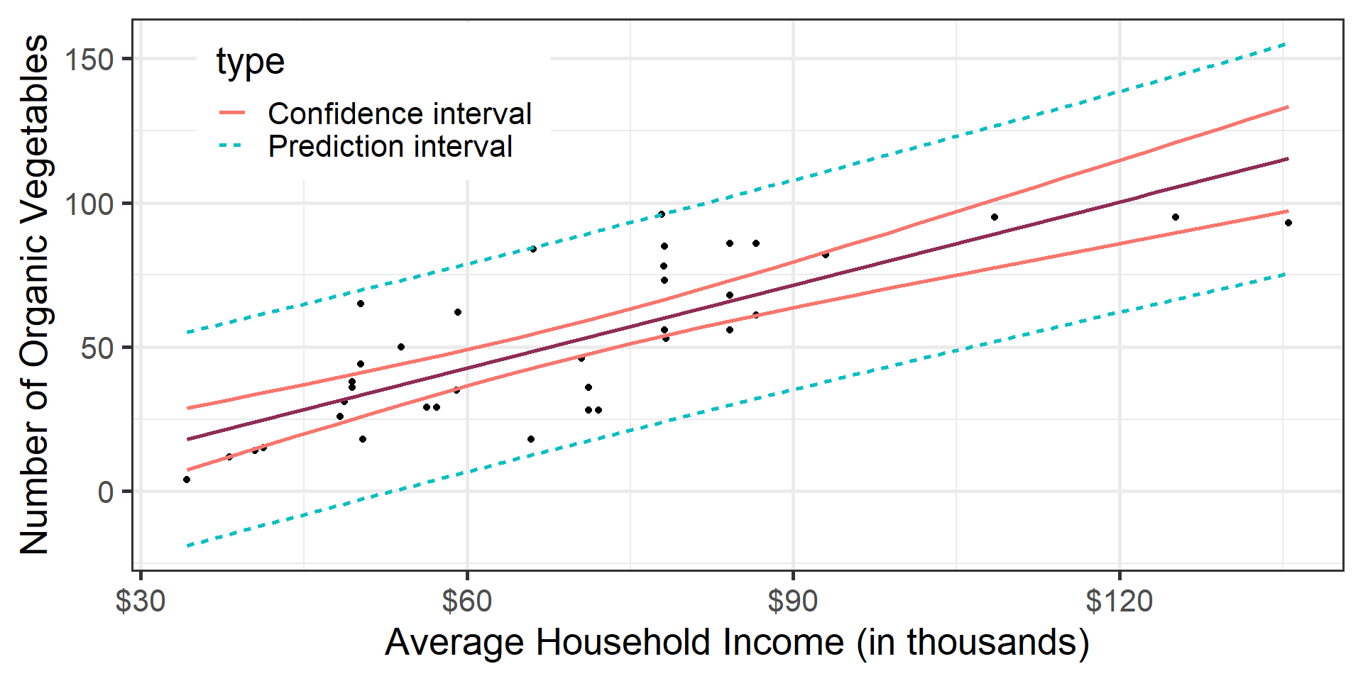
Comparing intervals

Extrapolation

Using the model to predict for values outside the range of the original data is extrapolation.

Calculate the prediction interval for the number of organic options in an extremely wealthy neighborhood with an average household income of $500k.

No, thanks!

Extrapolation

Why do we want to avoid extrapolation?