Multiple linear regression (MLR)

Prof. Eric Friedlander

Sep 30, 2024

Trying something new

• Open but do not start AE-10
• Notify Dr. F when you’re ready to proceed
• The goal is to integrate the activity into the lecture (keep track of how you like this approach and give Dr. F feedback at the end of class)
• While you’re waiting feel free to start on Exercise 0

📋 AE 10 - Credit Cards

Computational setup

# load packages
library(tidyverse)
library(broom)
library(mosaic)
library(ISLR2)
library(patchwork)
library(knitr)
library(kableExtra)
library(scales)

# set default theme and larger font size for ggplot2
ggplot2::theme_set(ggplot2::theme_minimal(base_size = 16))

Considering multiple variables

Data: Credit Cards

The data is from the Credit data set in the ISLR2 R package. It is a simulated data set of 400 credit card customers.

Rows: 400
Columns: 11
$ Income    <dbl> 14.891, 106.025, 104.593, 148.924, 55.882, 80.180, 20.996, 7…
$ Limit     <dbl> 3606, 6645, 7075, 9504, 4897, 8047, 3388, 7114, 3300, 6819, …
$ Rating    <dbl> 283, 483, 514, 681, 357, 569, 259, 512, 266, 491, 589, 138, …
$ Cards     <dbl> 2, 3, 4, 3, 2, 4, 2, 2, 5, 3, 4, 3, 1, 1, 2, 3, 3, 3, 1, 2, …
$ Age       <dbl> 34, 82, 71, 36, 68, 77, 37, 87, 66, 41, 30, 64, 57, 49, 75, …
$ Education <dbl> 11, 15, 11, 11, 16, 10, 12, 9, 13, 19, 14, 16, 7, 9, 13, 15,…
$ Own       <fct> No, Yes, No, Yes, No, No, Yes, No, Yes, Yes, No, No, Yes, No…
$ Student   <fct> No, Yes, No, No, No, No, No, No, No, Yes, No, No, No, No, No…
$ Married   <fct> Yes, Yes, No, No, Yes, No, No, No, No, Yes, Yes, No, Yes, Ye…
$ Region    <fct> South, West, West, West, South, South, East, West, South, Ea…
$ Balance   <dbl> 333, 903, 580, 964, 331, 1151, 203, 872, 279, 1350, 1407, 0,…

Variables

Features (another name for predictors)

• Income: Annual income (in 1000’s of US dollars)
• Rating: Credit Rating

Outcome

• Limit: Credit limit

Complete Exercises 0-1. Please don’t look ahead in the slides.

Outcome: Limit

Credit |> 
  gf_density(~Limit, fill = "steelblue") |> 
  gf_labs(title = "Distribution of credit limit",
          x = "Credit Limit")|> 
  gf_refine(scale_x_continuous(labels = dollar_format()))

	min	Q1	median	Q3	max	mean	sd	n	missing
	855	3088	4622.5	5872.75	13913	4735.6	2308.199	400	0

Predictors

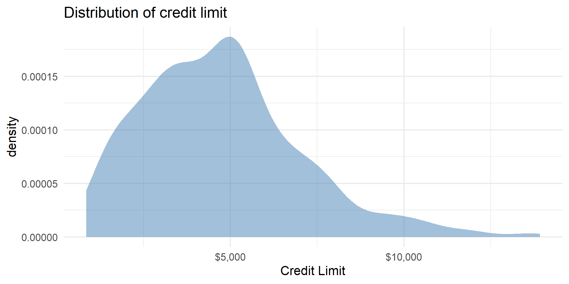
p1 <- Credit |> 
  gf_density(~Limit, fill = "steelblue") |> 
  gf_labs(title = "Distribution of credit limit",
          x = "Credit Limit")|> 
    gf_refine(scale_x_continuous(labels = dollar_format()))

p2 <- Credit |> 
  gf_histogram(~Rating, binwidth = 50) |> 
  gf_labs(title = "",
       x = "Credit Rating")

p3 <- Credit |> 
  gf_histogram(~Income, binwidth = 10) |> 
  gf_labs(title = "",
       x = "Annual income (in $1,000s)") |> 
  gf_refine(scale_x_continuous(labels = dollar_format()))

p1 / (p2 + p3)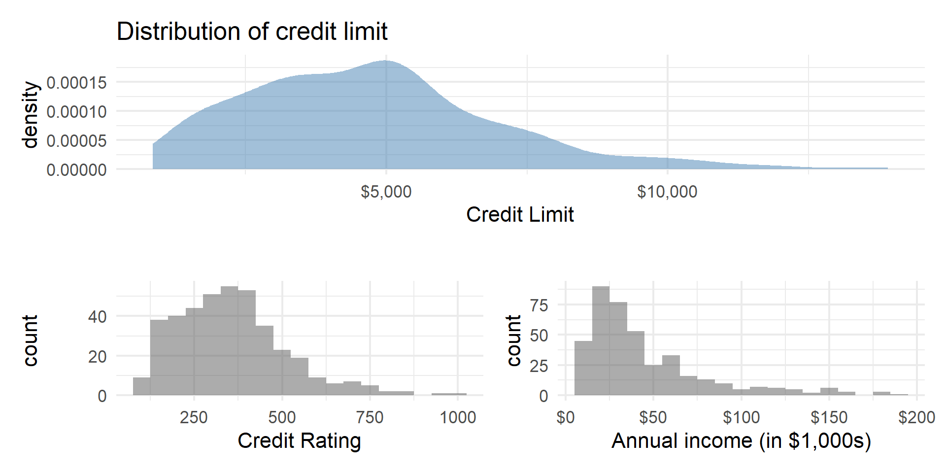

Outcome vs. predictors

p4 <- Credit |> 
  gf_point(Limit ~ Rating, color = "steelblue") |> 
  gf_labs(
    y = "Credit Limit",
    x = "Credit Rating"
  ) |> 
  gf_refine(scale_y_continuous(labels = dollar_format()))


p5 <- Credit |> 
  gf_point(Limit ~ Income, color = "steelblue") |> 
  gf_labs(
    y = "Credit Limit",
    x = "Annual income (in $1,000s)"
  ) |> 
  gf_refine(scale_x_continuous(labels = dollar_format()),
                               scale_y_continuous(labels = percent_format(scale = 1)))

p4 / p5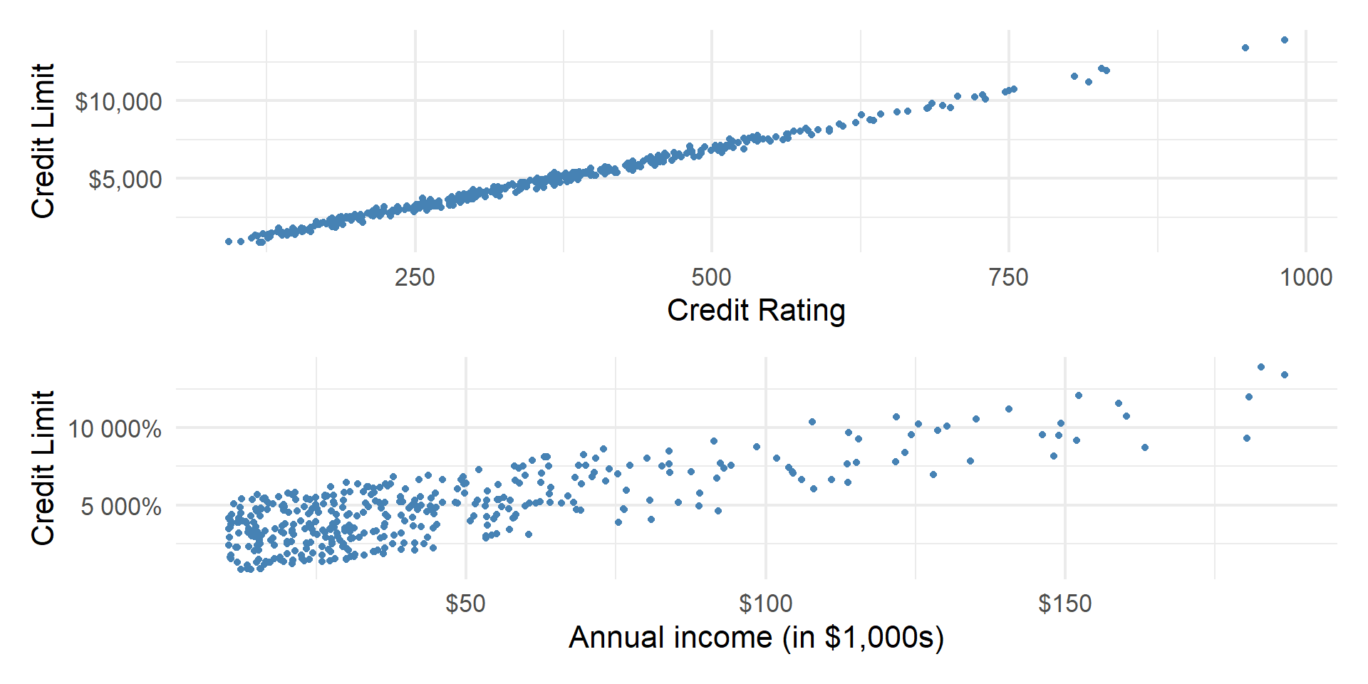

Single vs. multiple predictors

So far we’ve used a single predictor variable to understand variation in a quantitative response variable

Now we want to use multiple predictor variables to understand variation in a quantitative response variable

Multiple linear regression

Multiple linear regression (MLR)

Based on the analysis goals, we will use a multiple linear regression model of the following form

\[ \begin{aligned}\hat{\text{Limit}} ~ = \hat{\beta}_0 & + \hat{\beta}_1 \text{Rating} + \hat{\beta}_2 \text{Income} \end{aligned} \]

Similar to simple linear regression, this model assumes that at each combination of the predictor variables, the values Limit follow a Normal distribution.

Multiple linear regression

Recall: The simple linear regression model assumes

\[ Y|X\sim N(\beta_0 + \beta_1 X, \sigma_{\epsilon}^2) \]

Similarly: The multiple linear regression model assumes

\[ Y|X_1, X_2, \ldots, X_p \sim N(\beta_0 + \beta_1 X_1 + \beta_2 X_2 + \dots + \beta_p X_p, \sigma_{\epsilon}^2) \]

Multiple linear regression

At any combination of the predictors, the mean value of the response \(Y\), is

\[ \mu_{Y|X_1, \ldots, X_p} = \beta_0 + \beta_1 X_{1} + \beta_2 X_2 + \dots + \beta_p X_p \]

Using multiple linear regression, we can estimate the mean response for any combination of predictors

\[ \hat{Y} = \hat{\beta}_0 + \hat{\beta}_1 X_{1} + \hat{\beta}_2 X_2 + \dots + \hat{\beta}_p X_{p} \]

Model fit

Complete exercises 2-4 in the application exercise. Don’t look ahead!

Model fit

term	estimate	std.error	statistic	p.value
(Intercept)	-532.471	24.173	-22.028	0.000
Rating	14.771	0.096	153.124	0.000
Income	0.557	0.423	1.316	0.189

Model equation

\[ \begin{align}\hat{\text{Limit}} = -532.471 &+14.771 \times \text{Rating}\\ & -0.557 \times \text{Income} \end{align} \]

Interpreting \(\hat{\beta}_j\)

• The estimated coefficient \(\hat{\beta}_j\) is the expected change in the mean of \(y\) when \(x_j\) increases by one unit, holding the values of all other predictor variables constant.

Complete Exercises 5-6.

Prediction

What is the predicted credit limit for an borrower with an credit rating of ratio of 700, and who has an annual income of $59,000?

-532.471 + 14.771 * 700 + - .577 * 59

[1] 9773.186

The predicted credit limit for an borrower with an credit rating of ratio of 700, and who has an annual income of $59,000 is $9773.19.

Prediction, revisited

Just like with simple linear regression, we can use the predict function in R to calculate the appropriate intervals for our predicted values:

       fit      lwr      upr
1 9840.213 9476.983 10203.44

Note

Difference in predicted value due to rounding the coefficients on the previous slide.

Prediction interval for \(\hat{y}\)

Calculate a 90% confidence interval for the predicted credit limit for an individual borrower an credit rating of ratio of 700, and who has an annual income of $59,000?

predict(lim_fit, new_borrower, interval = "prediction", level = 0.90)

       fit      lwr      upr
1 9840.213 9535.599 10144.83

When would you use "confidence"? Would the interval be wider or narrower?

Cautions

• Do not extrapolate! Because there are multiple predictor variables, there is the potential to extrapolate in many directions
• The multiple regression model only shows association, not causality
  • To show causality, you must have a carefully designed experiment or carefully account for confounding variables in an observational study