# load packageslibrary(tidyverse)library(broom)library(ggformula)library(openintro)library(knitr)library(kableExtra) # for table embellishmentslibrary(Stat2Data) # for empirical logitlibrary(countdown)# set default theme and larger font size for ggplot2ggplot2::theme_set(ggplot2::theme_bw(base_size =20))
Data
Risk of coronary heart disease
This data set is from an ongoing cardiovascular study on residents of the town of Framingham, Massachusetts. We want to examine the relationship between various health characteristics and the risk of having heart disease.
TenYearCHD:
1: High risk of having heart disease in next 10 years
0: Not high risk of having heart disease in next 10 years
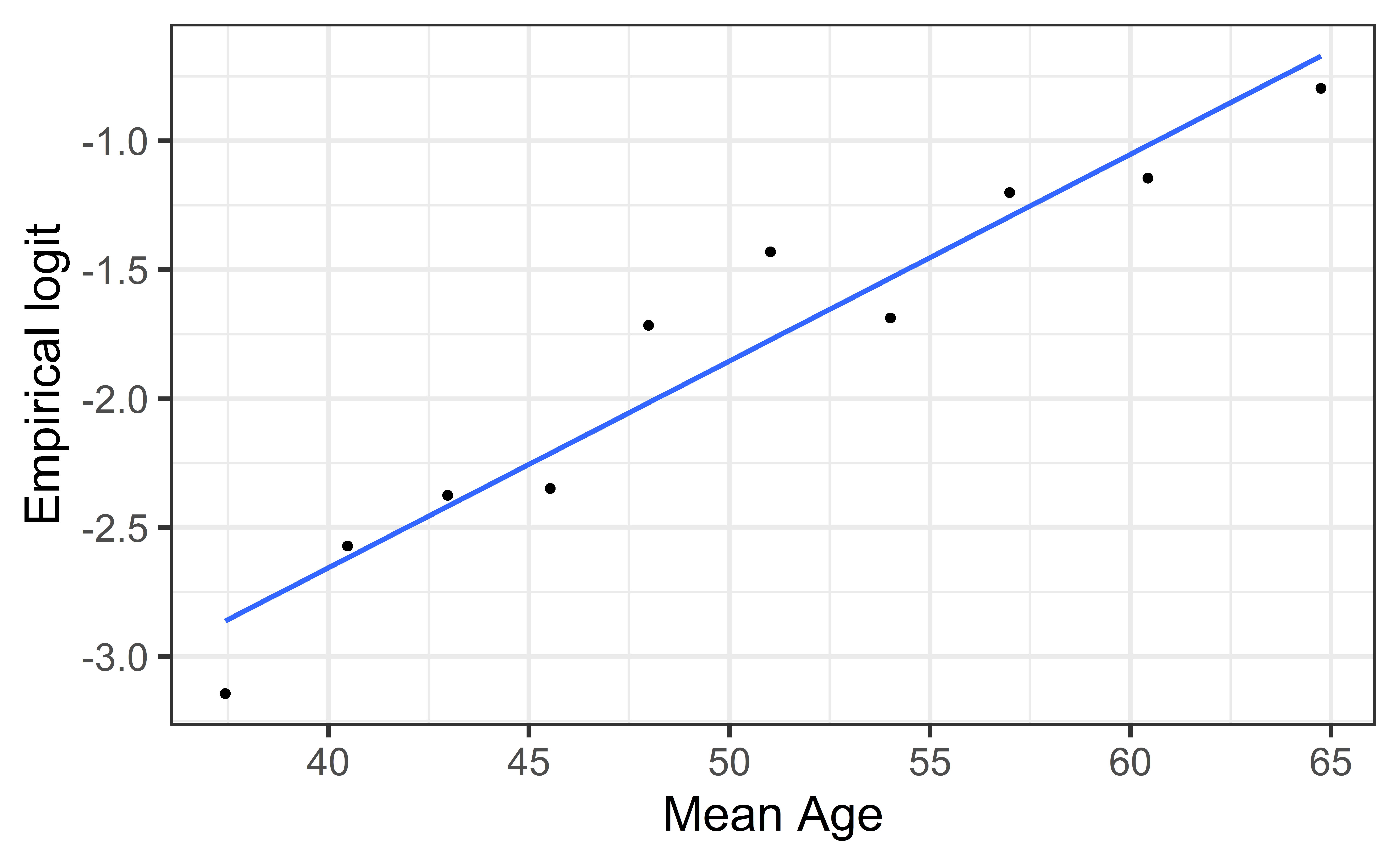
Divide the range of the predictor into intervals with approximately equal number of cases. (If you have enough observations, use 5 - 10 intervals.)
Compute the empirical logit for each interval
You can then calculate the mean value of the predictor in each interval and create a plot of the empirical logit versus the mean value of the predictor in each interval.
Empirical logit plot in R (quantitative predictor)
Created using dplyr and ggplot functions.
Empirical logit plot in R (quantitative predictor)
Created using dplyr and ggformula functions.
heart_disease |>mutate(age_bin =cut_interval(age, n =10)) |>group_by(age_bin) |>mutate(mean_age =mean(age)) |>count(mean_age, TenYearCHD) |>mutate(prop = n/sum(n)) |>filter(TenYearCHD =="1") |>mutate(emp_logit =log(prop/(1-prop))) |>gf_point(emp_logit ~ mean_age) |>gf_smooth(method ="lm", se =FALSE) |>gf_labs(x ="Mean Age", y ="Empirical logit")
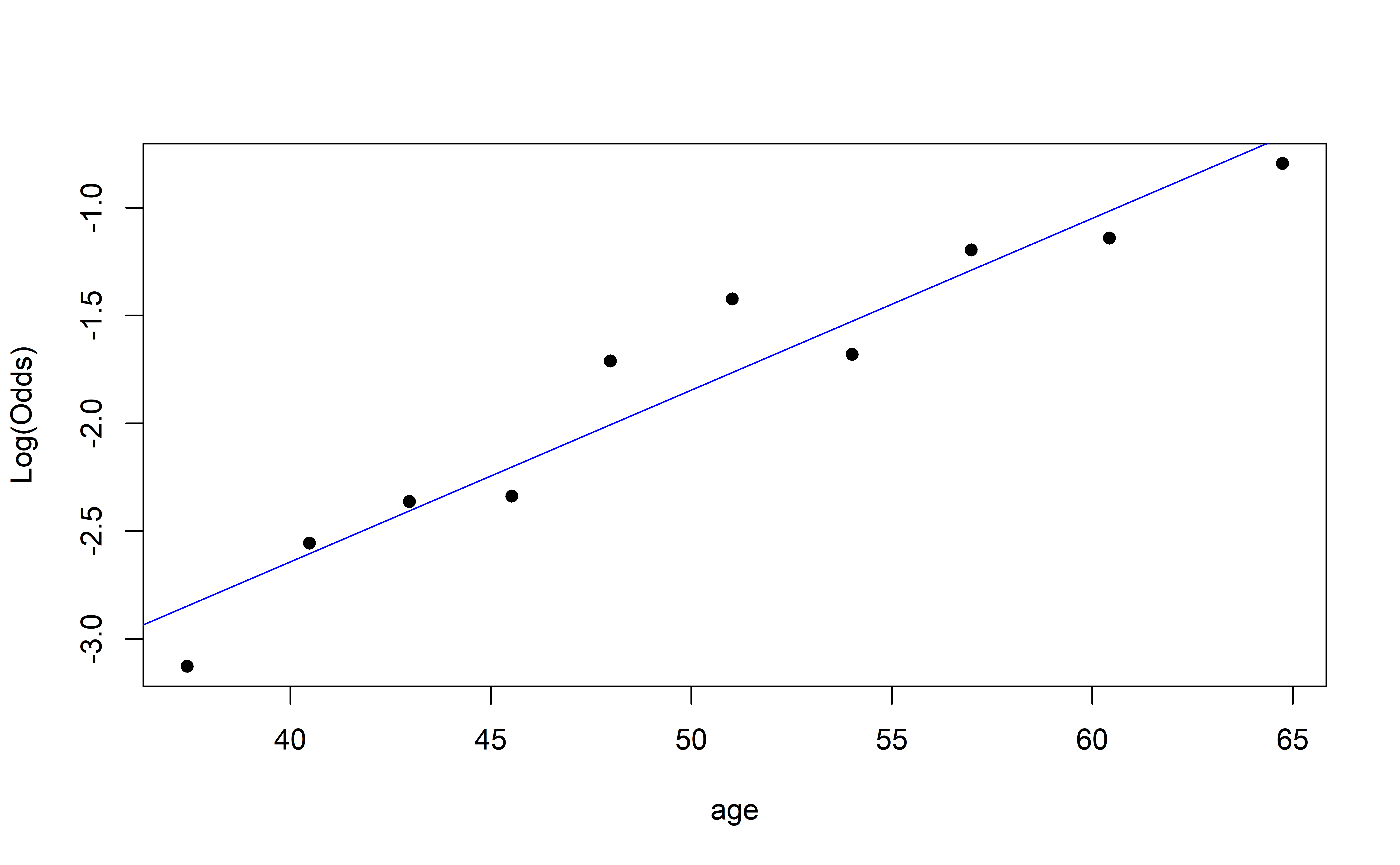
Empirical logit plot in R (quantitative predictor)
Using the emplogitplot1 function from the Stat2Data R package
emplogitplot1(TenYearCHD ~ age, data = heart_disease, ngroups =10)
Checking linearity
✅ The linearity condition is satisfied. There is a linear relationship between the empirical logit and the predictor variables.
Complete Exercise 3.
Checking randomness
We can check the randomness condition based on the context of the data and how the observations were collected.
Was the sample randomly selected?
If the sample was not randomly selected, ask whether there is reason to believe the observations in the sample differ systematically from the population of interest.
✅ The randomness condition is satisfied. We do not have reason to believe that the participants in this study differ systematically from adults in the U.S. in regards to health characteristics and risk of heart disease.
Checking independence
We can check the independence condition based on the context of the data and how the observations were collected.
Independence is most often violated if the data were collected over time or there is a strong spatial relationship between the observations.
✅ The independence condition is satisfied. It is reasonable to conclude that the participants’ health characteristics are independent of one another.
Recap
Logistic regression conditions
Linearity
Randomness
Independence
Rest of Class
Let’s start thinking about inference in the context of Logistic Regression. Find a spot on the white board with the rest of your group:
Design a simulation-based hypothesis test to determine whether your predictor is useful. Your answer should include a step by step guide of how to implement the test.
Design a simulation-based procedure for constructing a confidence interval for the coefficient of your assigned predictor.