Inference for Logistic Regression Models Continued
Nov 15, 2024
Do now
Write your confidence interval interpretations from Wednesday on the board.
Announcements
- Project: Paper Due November 18th
- Oral R Quiz
📋 AE 22 - Inference for Logistic Regression Models Continued
- Open up AE 22 and complete Exercise 0.
Topics
- Inference for coefficients in logistic regression
Computational setup
Data
Risk of coronary heart disease
This data set is from an ongoing cardiovascular study on residents of the town of Framingham, Massachusetts. We want to examine the relationship between various health characteristics and the risk of having heart disease.
TenYearCHD:- 1: Developed heart disease in next 10 years
- 0: Did not develop heart disease in next 10 years
age: Age at exam time (in years)
Data prep
Modeling risk of coronary heart disease
Using age:
Inference for Logistic Regression
Recall: Inference for Linear Regression
- t-test: determine whether \(\beta_1\) (the slope) is different than zero (Last Time)
- ANOVA/F-Test: To test the full model or to compare nested models
- SSModel/SSE/ \(R^2\) / \(\hat{\sigma}_{\epsilon}\) : metrics to try a measure the amount of variability explained by competing models
Recall: Likelihood
\[ L = \prod_{i=1}^n\hat{\pi}_i^{y_i}(1 - \hat{\pi}_i)^{1 - y_i} \]
- Intuition: probability of obtaining our data given a certain set of parameters
\[ L(\hat{\beta}_0, \ldots, \hat{\beta}_p) = \prod_{i=1}^n\hat{\pi}_i(\hat{\beta}_0, \ldots, \hat{\beta}_p)^{y_i}(1 - \hat{\pi}_i(\hat{\beta}_0, \ldots, \hat{\beta}_p))^{1 - y_i} \]
Recall: Log-Likelihood
Taking the log makes the likelihood easier to work with and doesn’t change which \(\beta\)’s maximize it.
\[ \log L = \sum\limits_{i=1}^n[y_i \log(\hat{\pi}_i) + (1 - y_i)\log(1 - \hat{\pi}_i)] \]
Log-Likelihood to Deviance
The log-likelihood measures of how well the model fits the data
Higher values of \(\log L\) are better
Deviance = \(-2 \log L\)
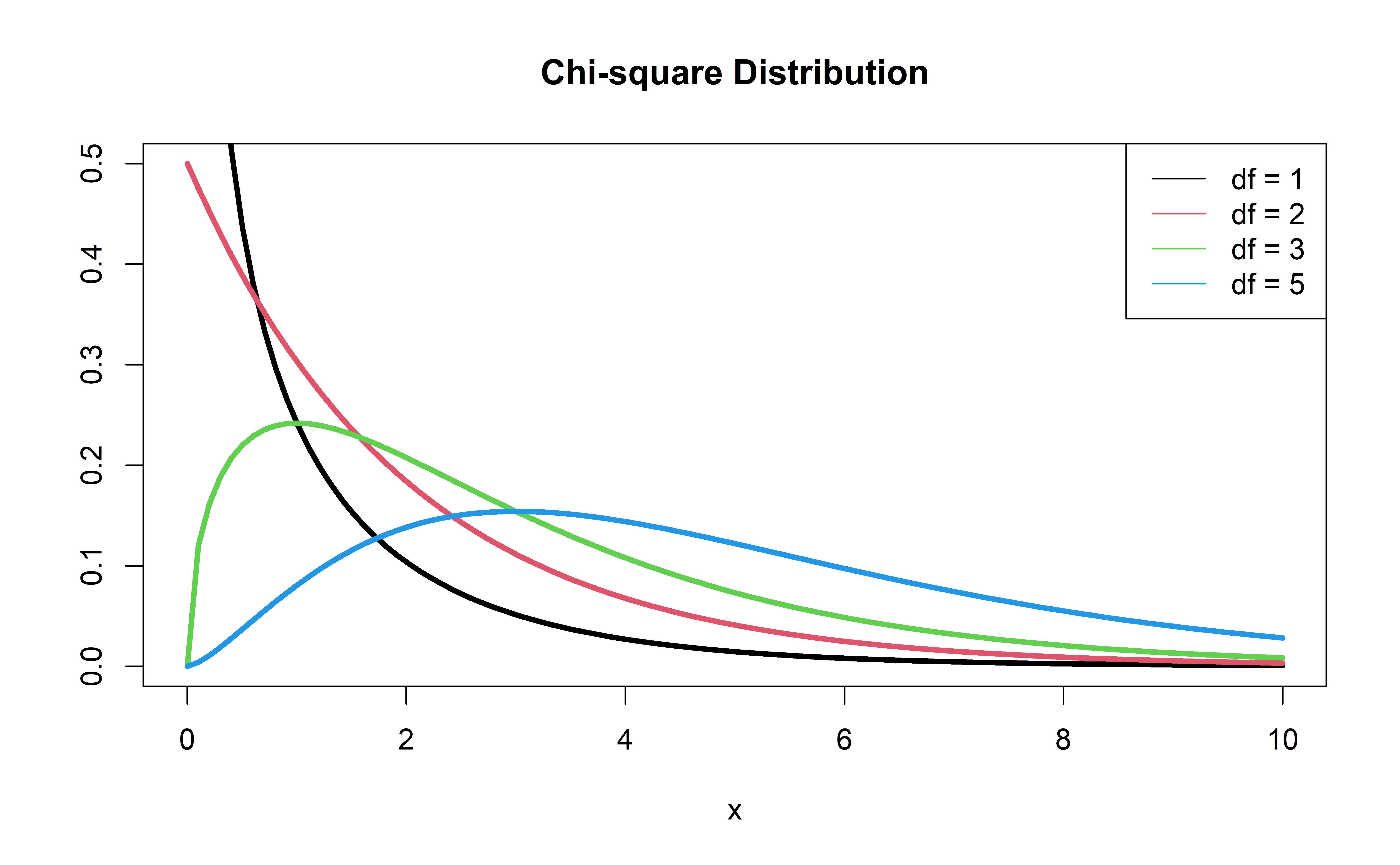
\(-2 \log L\) follows a \(\chi^2\) distribution with 1 degree of freedom
Think of deviace as the analog of the residual sum of squares (SSE) in linear regression
Calculate deviance for our model:
We can use our trusty ol’ glance function
| null.deviance | df.null | logLik | AIC | BIC | deviance | df.residual | nobs |
|---|---|---|---|---|---|---|---|
| 3612.209 | 4239 | -1698.305 | 3400.61 | 3413.314 | 3396.61 | 4238 | 4240 |
Complete Exercise 1.
Comparing nested models
Suppose there are two models:
- Reduced Model includes only an intercept \(\beta_0\)
- Full Model includes \(\beta_1\)
We want to test the hypotheses
\[ \begin{aligned} H_0&: \beta_{1} = 0\\ H_A&: \beta_1 \neq 0 \end{aligned} \]
To do so, we will use something called a Likelihood Ratio test (LRT), also known as the Drop-in-deviance test
Likelihood Ratio Test (LRT)
Hypotheses:
\[ \begin{aligned} H_0&: \beta_1 = 0 \\ H_A&: \beta_1 \neq 0 \end{aligned} \]
Test Statistic: \[G = (-2 \log L_{reduced}) - (-2 \log L_{full})\]
Sometimes written as \[G = (-2 \log L_0) - (-2 \log L)\]
P-value: \(P(\chi^2 > G)\), calculated using a \(\chi^2\) distribution with 1 degree of freedom
\(\chi^2\) distribution
Reduced model
First model, reduced:
Should we add age to the model?
Second model, full:
risk_fit_full <- glm(TenYearCHD ~ age,
      data = heart_disease, family = "binomial")

risk_fit_full |> tidy() |> kable()| term | estimate | std.error | statistic | p.value |
|---|---|---|---|---|
| (Intercept) | -5.5610898 | 0.2837460 | -19.59883 | 0 |
| age | 0.0746501 | 0.0052651 | 14.17821 | 0 |
Calculate deviance for each model:
Should we add age to the model?
Calculate the p-value using a pchisq(), with 1 degree of freedom:
Conclusion: The p-value is very small, so we reject \(H_0\). The data provide sufficient evidence that the coefficient of age is not equal to 0. Therefore, we should add it to the model.
Complete Exercises 2-3.
Drop-in-Deviance test in R
We can use the
anovafunction to conduct this testAdd
test = "Chisq"to conduct the drop-in-deviance test
Recap
Inference: Linear vs. Logistic Regression
- t-test: determine whether \(\beta_1\) (the slope) is different than zero
- ANOVA/F-Test: To test the full model or to compare nested models
- SSModel/SSE/ \(R^2\) / \(\hat{\sigma}_{\epsilon}\) : metrics to try and measure the amount of variability explained by competing models
Inference for \(\beta_1\)
- Last time: Wald Test
- Likelihood Ratio Test
- More reliable than Wald
- More computationally taxing
- Deviance: think of like SSE
- Next time: Multiple predictors!