Multiple Logistic Regression
Selection + Transformations
Dec 02, 2024
Recall: Empirical Logit Plot
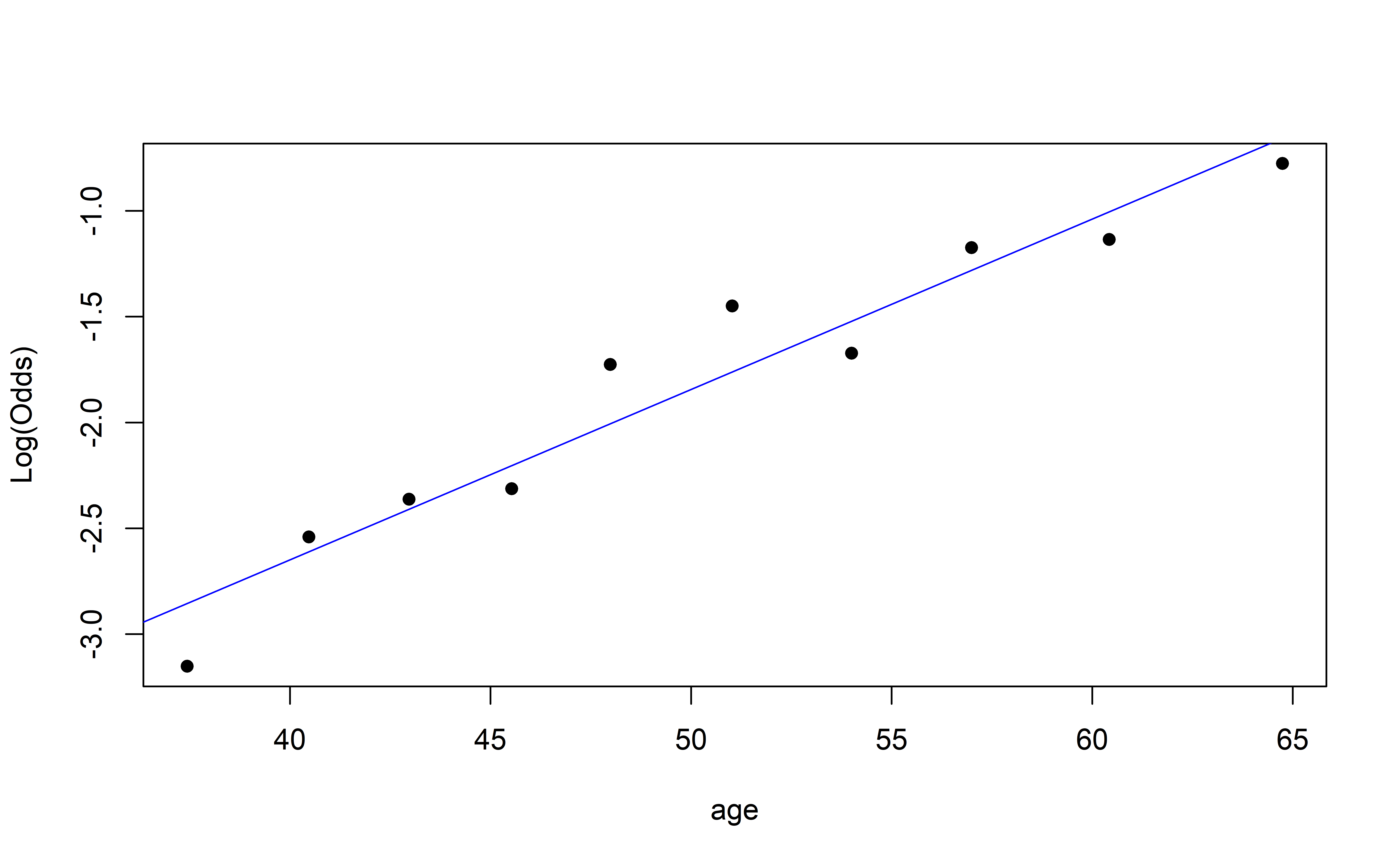
How do we interpret this?
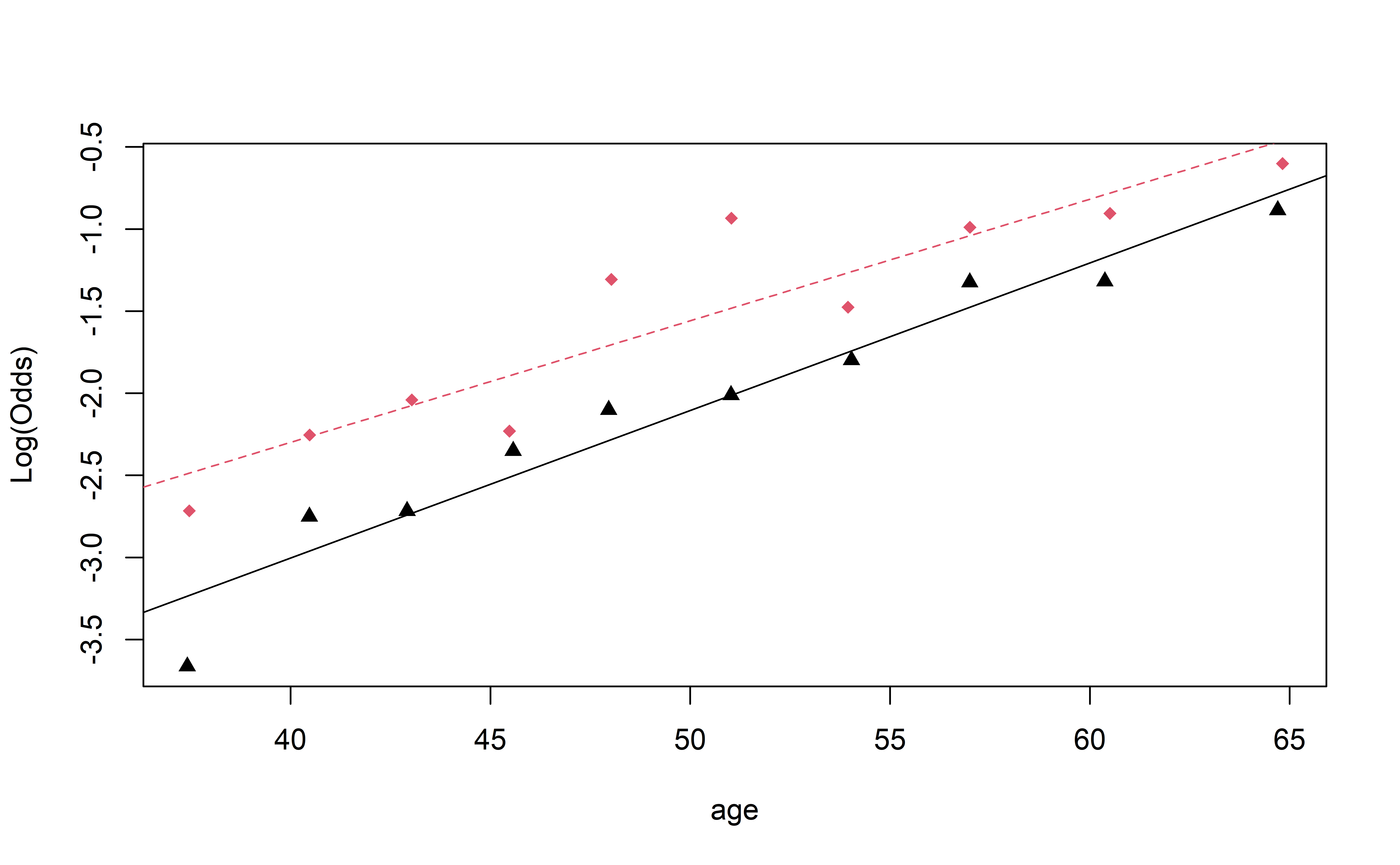
Visualizing Interactions (Quant vs. Cat)
Complete Exercise 2.
Visualizing Interactions (Quant vs. Cat)
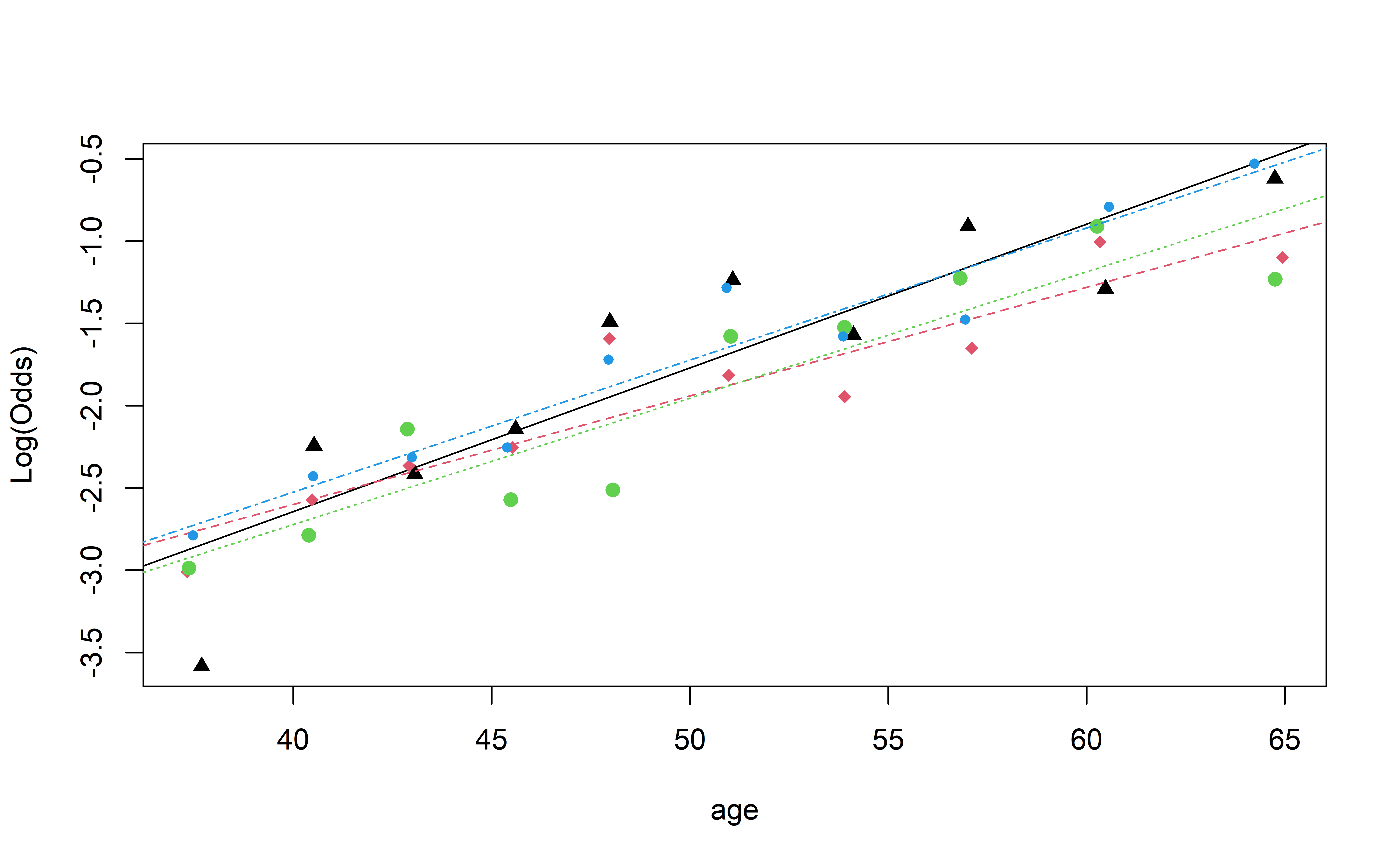
Based on this plot, do you think there is an interaction between age and education?
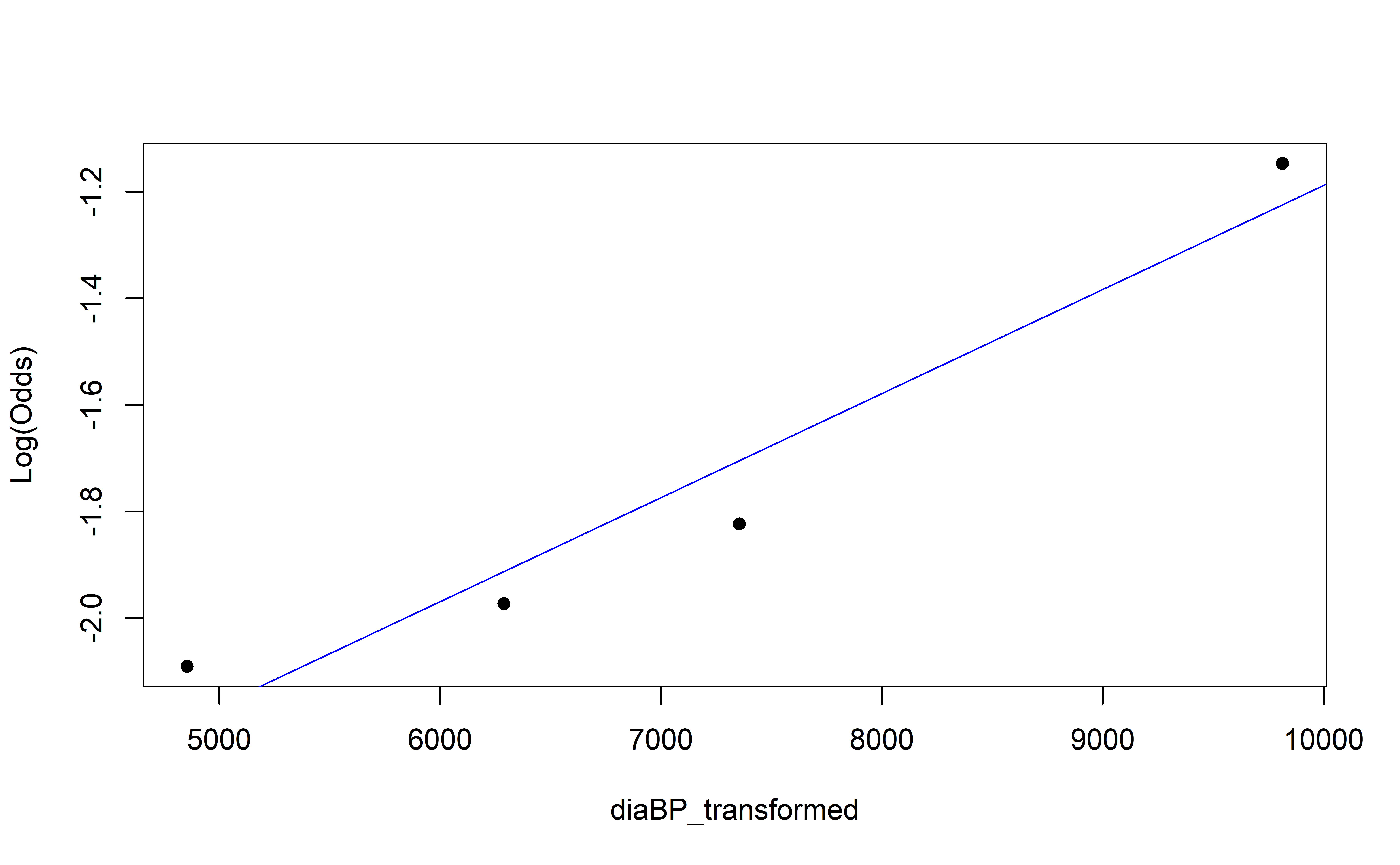
Empirical Log-Odds Plot

Empirical Log-Odds Plot
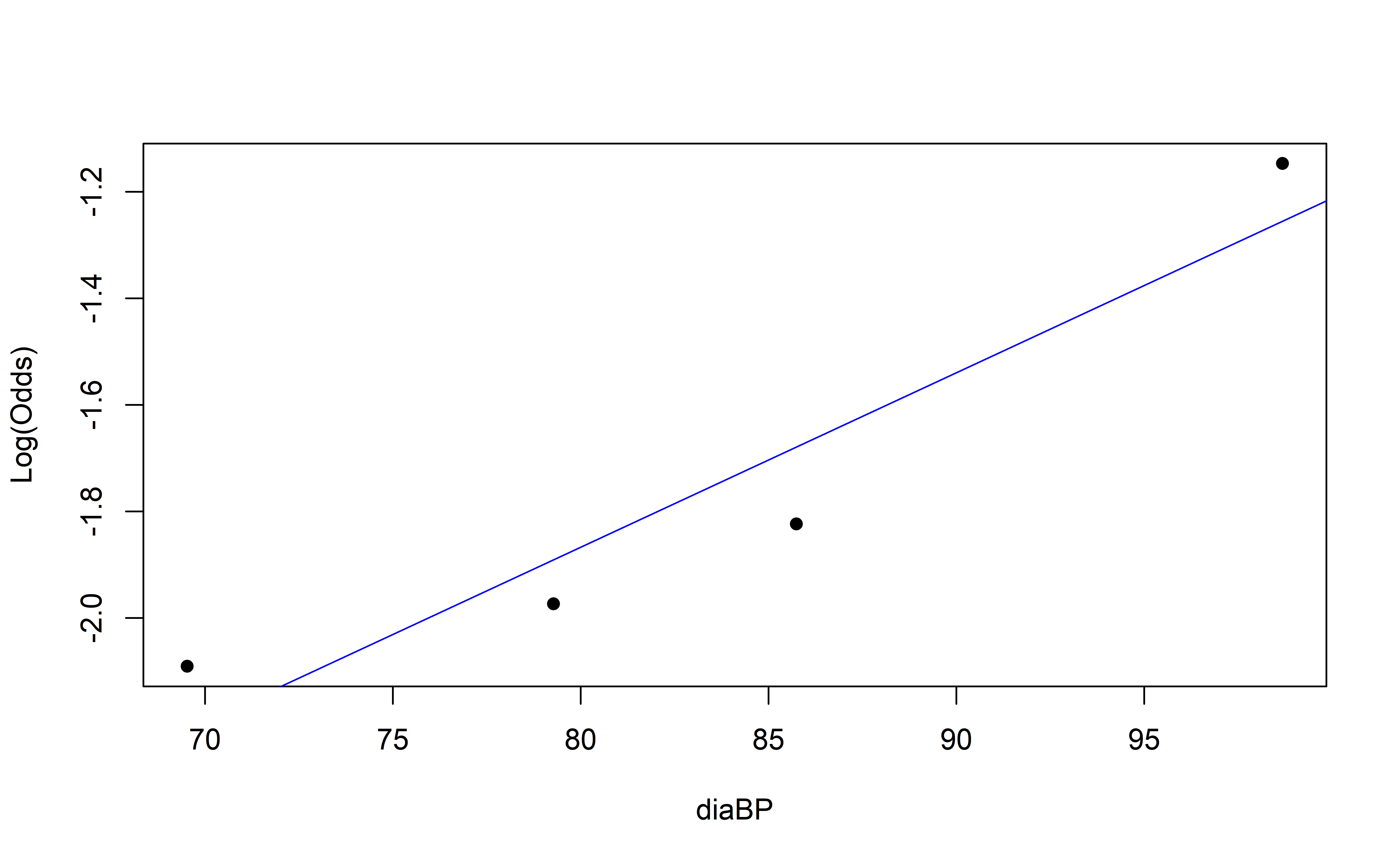
Concave up or down?
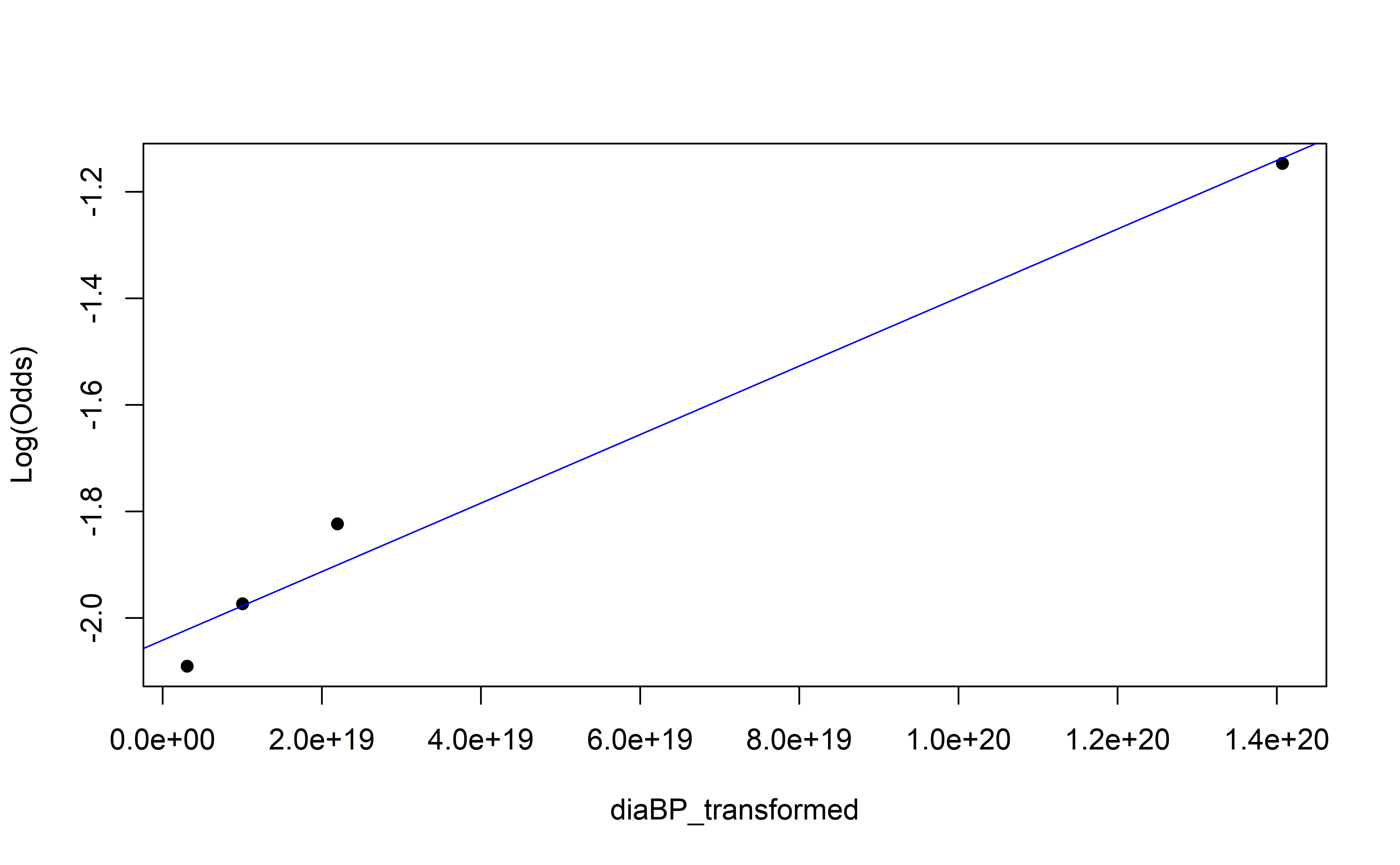
Empirical Log-Odds Plot
Empirical Log-Odds Plot
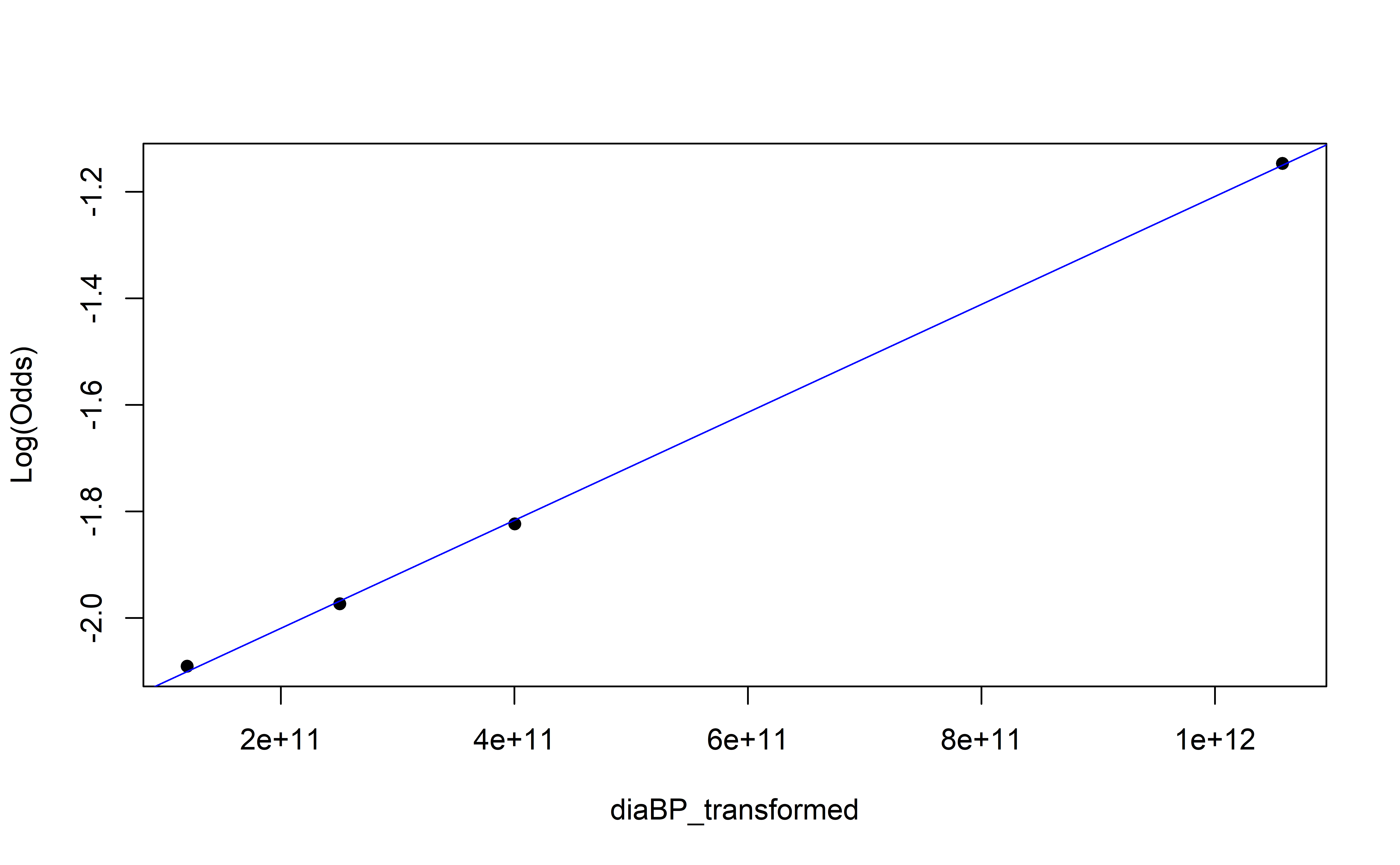
Empirical Log-Odds Plot
Recap
Interaction terms in logistic regression models
- For quantitative-categorical, creates nested models
Comparing logistic regression models
- AIC/BIC
Choosing logistic regression models
- Same selection techniques as linear regression
Transformations in logistic regression
Can only transform \(X\)
Concave [up/down] \(\Rightarrow\) power-transform [up/down]
![]()