# load packages
library(tidyverse)   # for data wrangling and visualization
library(broom)       # for nearly formatting model output
library(ggformula)   # for plotting
library(infer)       # for simulation based inference
library(scales)      # for pretty axis labels
library(knitr)       # for neatly formatted tables

# load my data
heb <- read_csv("data/HEBIncome.csv") |>
  mutate(Avg_Income_K = Avg_Household_Income/1000)


# set default theme and larger font size for ggplot2
ggplot2::theme_set(ggplot2::theme_bw(base_size = 16))SLR: Randomization test for the slope
Prof. Eric Friedlander
Sep 06, 2024
Application exercise
Concept Check
You professor is interested in calculating the average amount of time CofI students spend doing homework.
- If he collects a set of data and asks 100 students to compute 95% confidence intervals from that data, how many of those would you expect to contain the true average?
- If, instead, he has each of those 100 students collect their own data and compute 95% confidence intervals from their own data, how many would you expect to contain the true average?
From last time
Population: Complete set of observations of whatever we are studying, e.g., people, tweets, photographs, etc. (population size = \(N\))
Sample: Subset of the population, ideally random and representative (sample size = \(n\))
Sample statistic \(\ne\) population parameter, but if the sample is good, it can be a good estimate
Statistical inference: Discipline that concerns itself with the development of procedures, methods, and theorems that allow us to extract meaning and information from data that has been generated by stochastic (random) process
We report the estimate with a confidence interval, and the width of this interval depends on the variability of sample statistics from different samples from the population
Since we can’t continue sampling from the population, we bootstrap from the one sample we have to estimate sampling variability
Topics
Evaluate a claim about the slope using hypothesis testing
Define mathematical models to conduct inference for slope
Computational setup
Recap of last lecture
Data: San Antonio Income & Organic Food Access
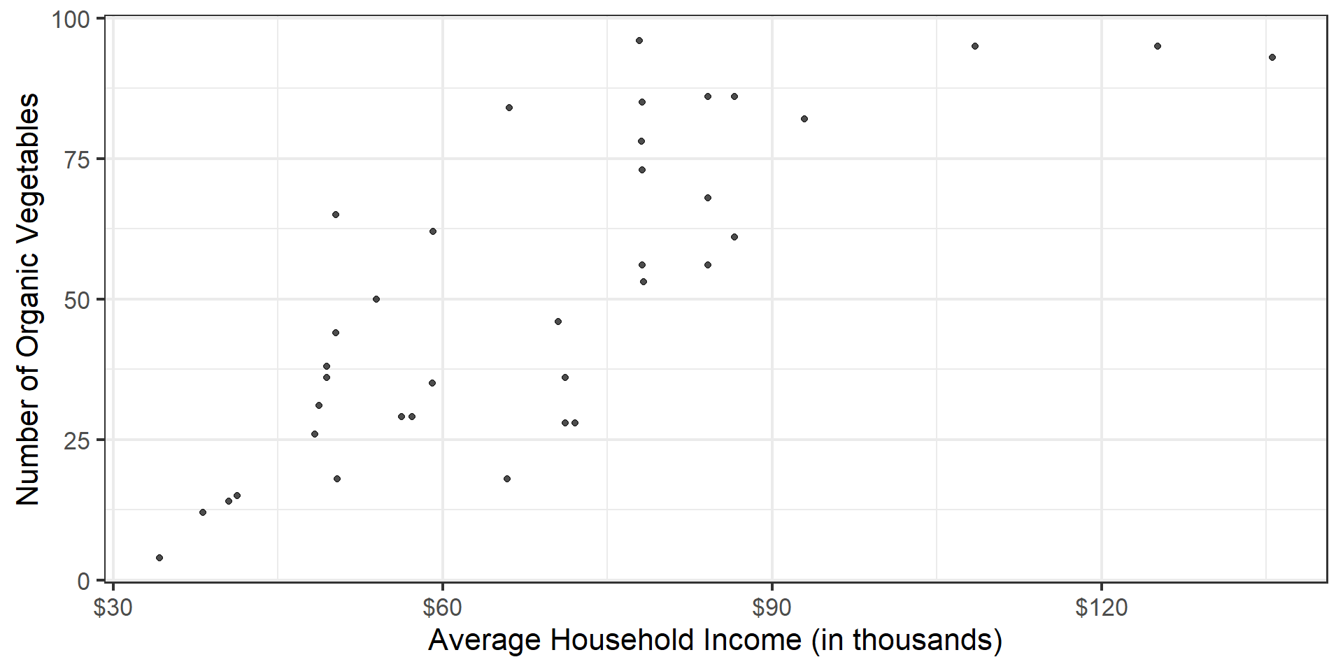
The regression model
| term | estimate | std.error | statistic | p.value |
|---|---|---|---|---|
| (Intercept) | -14.72 | 9.30 | -1.58 | 0.12 |
| Avg_Income_K | 0.96 | 0.13 | 7.50 | 0.00 |
Slope: For each additional $1,000 in average household income, we expect the number of organic options available at nearby HEBs to increase by 0.96, on average.
Inference for simple linear regression
Calculate a confidence interval for the slope, \(\beta_1\)
Conduct a hypothesis test for the slope, \(\beta_1\)
Sampling is natural

- When you taste a spoonful of soup and decide the spoonful you tasted isn’t salty enough, that’s exploratory analysis
- If you generalize and conclude that your entire soup needs salt, that’s an inference
- For your inference to be valid, the spoonful you tasted (the sample) needs to be representative of the entire pot (the population)
Confidence interval via bootstrapping
- Bootstrap new samples from the original sample
- Fit models to each of the samples and estimate the slope
- Use features of the distribution of the bootstrapped slopes to construct a confidence interval
Bootstrapping pipeline I
Response: Number_Organic (numeric)
Explanatory: Avg_Income_K (numeric)
# A tibble: 37 × 2
Number_Organic Avg_Income_K
<dbl> <dbl>
1 36 71.2
2 4 34.2
3 28 71.2
4 31 48.8
5 78 78.1
6 14 40.5
7 12 38.2
8 18 50.4
9 38 49.4
10 84 66.1
# ℹ 27 more rowsBootstrapping pipeline II
set.seed(212)

heb |>
specify(Number_Organic ~ Avg_Income_K) |>
generate(reps = 1000, type = "bootstrap")Response: Number_Organic (numeric)
Explanatory: Avg_Income_K (numeric)
# A tibble: 37,000 × 3
# Groups: replicate [1,000]
replicate Number_Organic Avg_Income_K
<int> <dbl> <dbl>
1 1 44 50.3
2 1 18 50.4
3 1 29 56.3
4 1 85 78.2
5 1 86 84.2
6 1 12 38.2
7 1 15 41.3
8 1 82 92.9
9 1 28 72.1
10 1 85 78.2
# ℹ 36,990 more rowsBootstrapping pipeline III
set.seed(212)
heb |>
specify(Number_Organic ~ Avg_Income_K) |>
generate(reps = 1000, type = "bootstrap") |>
fit()# A tibble: 2,000 × 3
# Groups: replicate [1,000]
replicate term estimate
<int> <chr> <dbl>
1 1 intercept -8.22
2 1 Avg_Income_K 0.869
3 2 intercept -8.52
4 2 Avg_Income_K 0.878
5 3 intercept -16.4
6 3 Avg_Income_K 0.948
7 4 intercept -38.2
8 4 Avg_Income_K 1.37
9 5 intercept -5.62
10 5 Avg_Income_K 0.836
# ℹ 1,990 more rowsBootstrapping pipeline IV
Visualize the bootstrap distribution
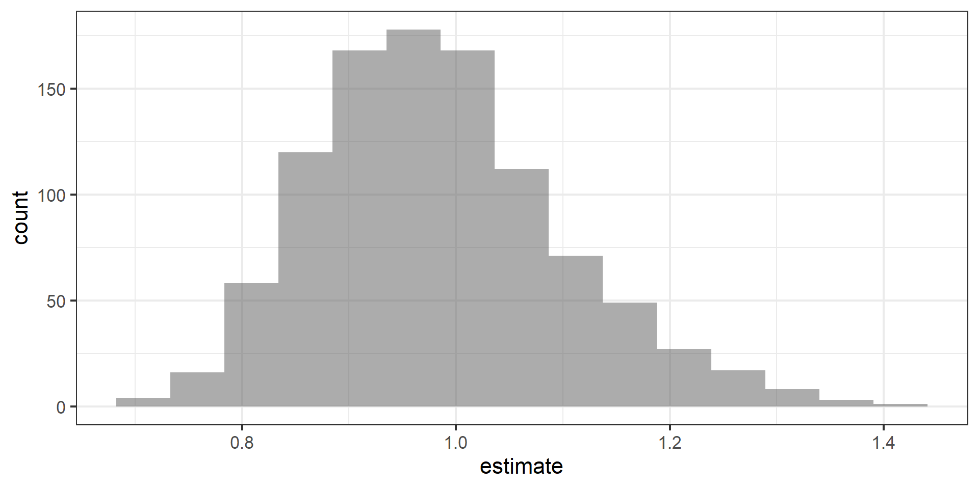
Compute the CI
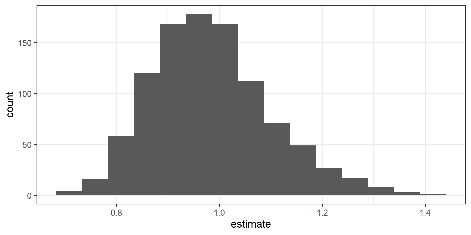
But first…
Compute 95% confidence interval
Hypothesis test for the slope
Research question and hypotheses
“Do the data provide sufficient evidence that \(\beta_1\) (the true slope for the population) is different from 0?”
Null hypothesis: there is no linear relationship between Number_Organic and Avg_Income_K
\[ H_0: \beta_1 = 0 \]
Alternative hypothesis: there is a linear relationship between Number_Organic and Avg_Income_K
\[ H_A: \beta_1 \ne 0 \]
Hypothesis testing as a court trial
- Null hypothesis, \(H_0\): Defendant is innocent
- Alternative hypothesis, \(H_A\): Defendant is guilty
- Present the evidence: Collect data
- Judge the evidence: “Could these data plausibly have happened by chance if the null hypothesis were true?”
- Yes: Fail to reject \(H_0\)
- No: Reject \(H_0\)
- Not guilty \(\neq\) innocent \(\implies\) why we say “fail to reject the null” rather than “accept the null”
Hypothesis testing framework
- Start with a null hypothesis, \(H_0\) that represents the status quo
- Set an alternative hypothesis, \(H_A\) that represents the research question, i.e. claim we’re testing
- Under the assumption that the null hypothesis is true, calculate a p-value (probability of getting outcome or outcome even more favorable to the alternative)
- if the test results suggest that the data do not provide convincing evidence for the alternative hypothesis, stick with the null hypothesis
- if they do, then reject the null hypothesis in favor of the alternative
Quantify the variability of the slope
for testing
- Two approaches:
- Via simulation
- Via mathematical models
- Use Randomization to quantify the variability of the slope for the purpose of testing, under the assumption that the null hypothesis is true:
- Simulate new samples from the original sample via permutation
- Fit models to each of the samples and estimate the slope
- Use features of the distribution of the permuted slopes to conduct a hypothesis test
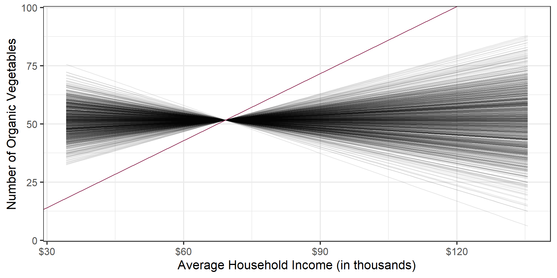
Permutation, described
- Use permuting to simulate data under the assumption the null hypothesis is true and measure the natural variability in the data due to sampling, not due to variables being correlated
- Permute reponse variable to eliminate any existing relationship with explanatory variable
- Each
Number_Organicvalue is randomly assigned to theAvg_Household_K, i.e.Number_OrganicandAvg_Household_Kare no longer matched for a given store
# A tibble: 37 × 3
Number_Organic_Original Number_Organic_Permuted Avg_Income_K
<dbl> <dbl> <dbl>
1 36 73 71.2
2 4 29 34.2
3 28 35 71.2
4 31 38 48.8
5 78 78 78.1
6 14 14 40.5
7 12 82 38.2
8 18 31 50.4
9 38 4 49.4
10 84 12 66.1
# ℹ 27 more rowsPermutation, visualized
- Each of the observed values for
area(and forprice) exist in both the observed data plot as well as the permutedpriceplot - Permuting removes the relationship between
areaandprice

Permutation, repeated
Repeated permutations allow for quantifying the variability in the slope under the condition that there is no linear relationship (i.e., that the null hypothesis is true)
Concluding the hypothesis test
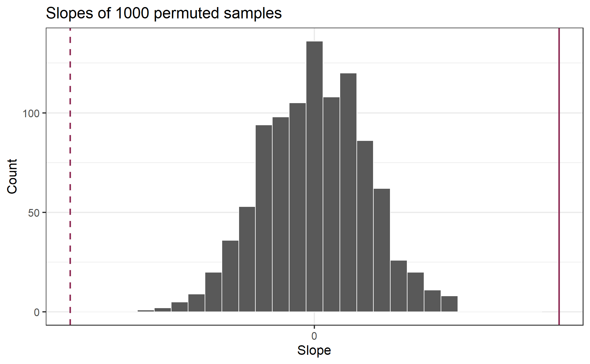
Is the observed slope of \(\hat{\beta_1} = 0.96\) (or an even more extreme slope) a likely outcome under the null hypothesis that \(\beta = 0\)? What does this mean for our original question: “Do the data provide sufficient evidence that \(\beta_1\) (the true slope for the population) is different from 0?”
Permutation pipeline I
Response: Number_Organic (numeric)
Explanatory: Avg_Income_K (numeric)
# A tibble: 37 × 2
   Number_Organic Avg_Income_K
            <dbl>        <dbl>
 1             36         71.2
 2              4         34.2
 3             28         71.2
 4             31         48.8
 5             78         78.1
 6             14         40.5
 7             12         38.2
 8             18         50.4
 9             38         49.4
10             84         66.1
# ℹ 27 more rowsPermutation pipeline II
Response: Number_Organic (numeric)
Explanatory: Avg_Income_K (numeric)
Null Hypothesis: independence
# A tibble: 37 × 2
Number_Organic Avg_Income_K
<dbl> <dbl>
1 36 71.2
2 4 34.2
3 28 71.2
4 31 48.8
5 78 78.1
6 14 40.5
7 12 38.2
8 18 50.4
9 38 49.4
10 84 66.1
# ℹ 27 more rowsPermutation pipeline III
set.seed(1218)

heb |>
specify(Number_Organic ~ Avg_Income_K) |>
hypothesize(null = "independence") |>
generate(reps = 1000, type = "permute")Response: Number_Organic (numeric)
Explanatory: Avg_Income_K (numeric)
Null Hypothesis: independence
# A tibble: 37,000 × 3
# Groups: replicate [1,000]
Number_Organic Avg_Income_K replicate
<dbl> <dbl> <int>
1 38 71.2 1
2 56 34.2 1
3 28 71.2 1
4 14 48.8 1
5 29 78.1 1
6 36 40.5 1
7 84 38.2 1
8 18 50.4 1
9 96 49.4 1
10 26 66.1 1
# ℹ 36,990 more rowsPermutation pipeline IV
set.seed(1218)

heb |>
  specify(Number_Organic ~ Avg_Income_K) |>
hypothesize(null = "independence") |>
generate(reps = 1000, type = "permute") |>
fit()# A tibble: 2,000 × 3
# Groups: replicate [1,000]
replicate term estimate
<int> <chr> <dbl>
1 1 intercept 47.8
2 1 Avg_Income_K 0.0555
3 2 intercept 58.0
4 2 Avg_Income_K -0.0914
5 3 intercept 57.3
6 3 Avg_Income_K -0.0817
7 4 intercept 78.9
8 4 Avg_Income_K -0.394
9 5 intercept 34.8
10 5 Avg_Income_K 0.244
# ℹ 1,990 more rowsPermutation pipeline V
Visualize the null distribution
Reason around the p-value
In a world where the there is no relationship between the the number of organic food options and the nearby average household income (\(\beta_1 = 0\)), what is the probability that we observe a sample of 37 stores where the slope fo the model predicting the number of organic options from average household income is 0.96 or even more extreme?
Compute the p-value
What does this warning mean?
Warning: Please be cautious in reporting a p-value of 0. This result is an approximation
based on the number of `reps` chosen in the `generate()` step.
ℹ See `get_p_value()` (`?infer::get_p_value()`) for more information.
Please be cautious in reporting a p-value of 0. This result is an approximation
based on the number of `reps` chosen in the `generate()` step.
ℹ See `get_p_value()` (`?infer::get_p_value()`) for more information.
# A tibble: 2 × 2
term p_value
<chr> <dbl>
1 Avg_Income_K 0
2 intercept 0