SLR: Conditions

Prof. Eric Friedlander

Sep 13, 2024

Application exercise

Questions from last class?

Computational set up

# load packages
library(tidyverse)   # for data wrangling and visualization
library(ggformula)   # for plotting using formulas
library(broom)       # for formatting model output
library(scales)      # for pretty axis labels
library(knitr)       # for pretty tables
library(kableExtra)  # also for pretty tables
library(patchwork)   # arrange plots

# HEB Dataset
heb <- read_csv("data/HEBIncome.csv") |> 
  mutate(Avg_Income_K = Avg_Household_Income/1000)

# set default theme and larger font size for ggplot2
ggplot2::theme_set(ggplot2::theme_bw(base_size = 20))

Regression model, revisited

heb_fit <- lm(Number_Organic ~ Avg_Income_K, data = heb)

tidy(heb_fit) |>
  kable(digits = 3)

term	estimate	std.error	statistic	p.value
(Intercept)	-14.719	9.298	-1.583	0.122
Avg_Income_K	0.959	0.128	7.505	0.000

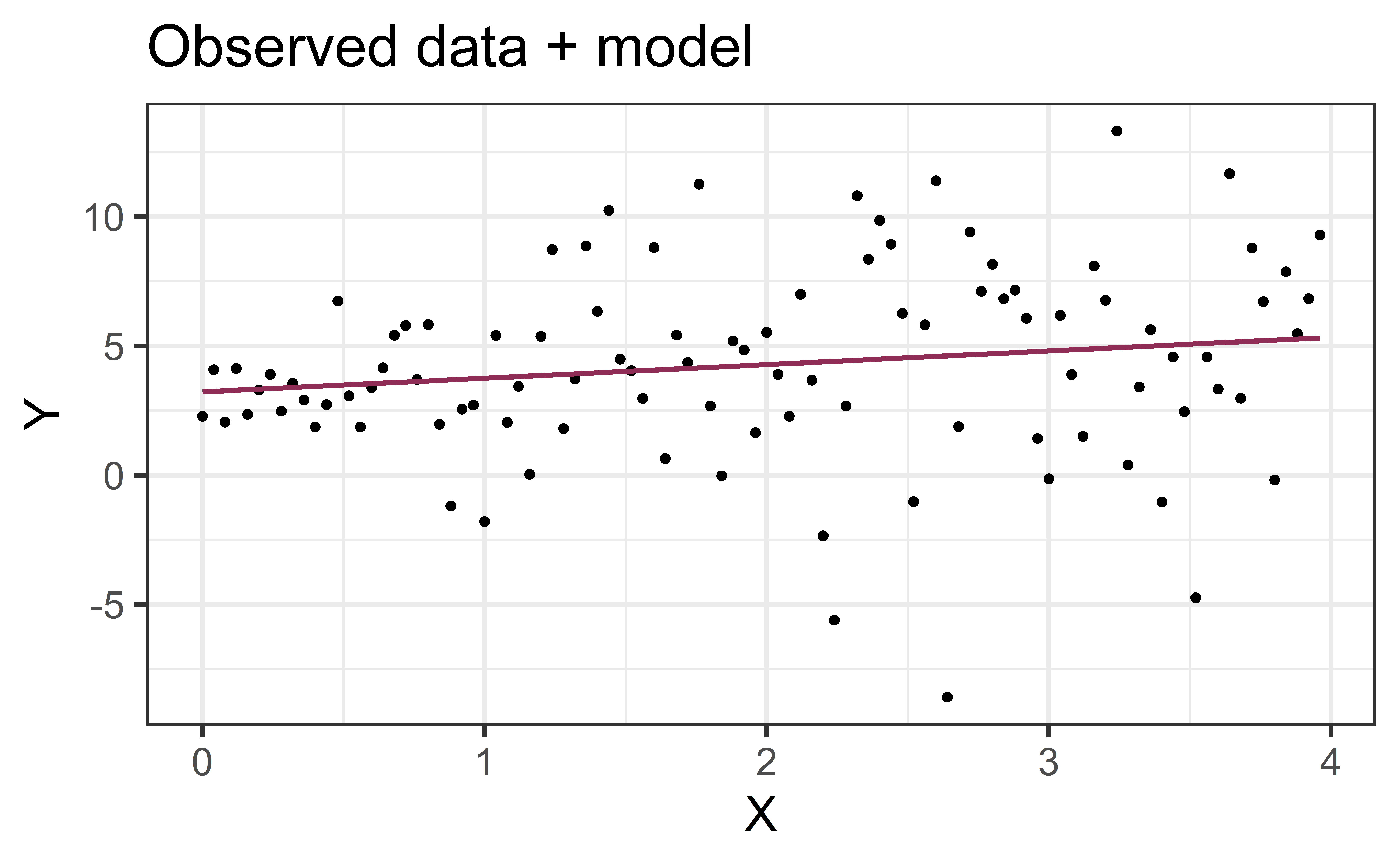
Mathematical representation, visualized

\[ Y|X \sim N(\beta_0 + \beta_1 X, \sigma_\epsilon^2) \]

Image source: Introduction to the Practice of Statistics (5th ed)

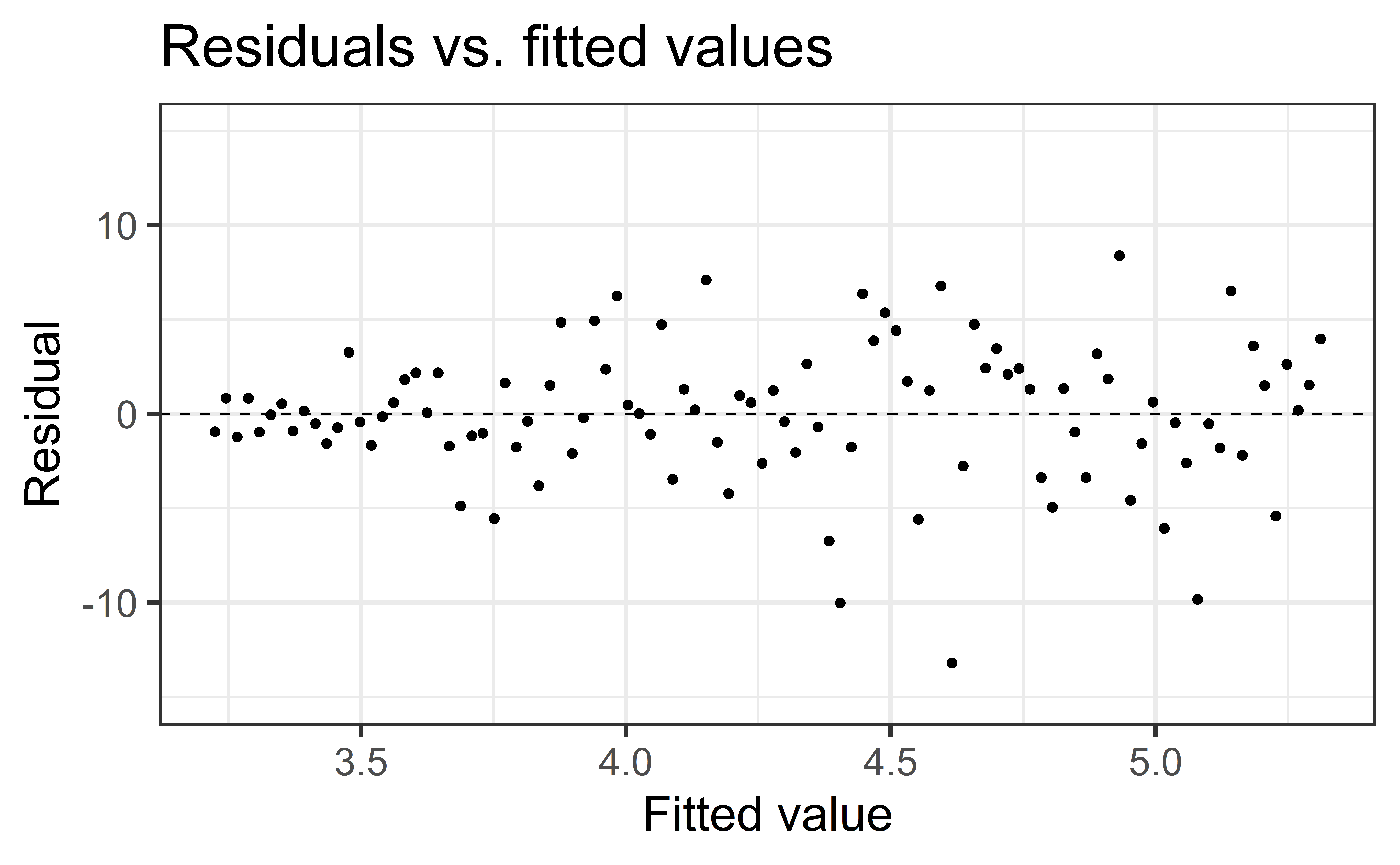
Model conditions

Linearity: There is a linear relationship between the outcome and predictor variables
Constant variance: The variability of the errors is equal for all values of the predictor variable
Normality: The errors follow a normal distribution
Independence: The errors are independent from each other

Linearity

If the linear model, \(\hat{y}_i = \hat{\beta}_0 + \hat{\beta}_1x_i\), adequately describes the relationship between \(X\) and \(Y\), then the residuals should reflect random (chance) error
To assess this, we can look at a plot of the residuals vs. the fitted values
Linearity satisfied if there is no distinguishable pattern in the residuals plot, i.e. the residuals should be randomly scattered
A non-random pattern (e.g. a parabola) suggests a linear model does not adequately describe the relationship between \(X\) and \(Y\)

Linearity

✅ The residuals vs. fitted values plot should show a random scatter of residuals (no distinguishable pattern or structure)

The augment function

heb_aug <- augment(heb_fit)

head(heb_aug) |> kable()

Number_Organic	Avg_Income_K	.fitted	.resid	.hat	.sigma	.cooksd	.std.resid
36	71.186	53.55498	-17.554983	0.0272386	17.45293	0.0145449	-1.0192493
4	34.234	18.11468	-14.114677	0.0925015	17.53471	0.0366889	-0.8484596
28	71.186	53.55498	-25.554983	0.0272386	17.15160	0.0308219	-1.4837325
31	48.760	32.04642	-1.046423	0.0493994	17.71691	0.0000981	-0.0614599
78	78.096	60.18230	17.817702	0.0312671	17.44374	0.0173428	1.0366517
14	40.506	24.13009	-10.130092	0.0711183	17.62593	0.0138683	-0.6018889

Residuals vs. fitted values (code)

heb_aug <- augment(heb_fit)

gf_point(.resid ~ .fitted, data = heb_aug) |> 
  gf_hline(yintercept = 0, linetype = "dashed") |> 
  gf_labs(
    x = "Fitted value", y = "Residual",
    title = "Residuals vs. fitted values"
  )

Non-linear relationships

Constant variance

If the spread of the distribution of \(Y\) is equal for all values of \(X\) then the spread of the residuals should be approximately equal for each value of \(X\)
To assess this, we can look at a plot of the residuals vs. the fitted values
Constant variance satisfied if the vertical spread of the residuals is approximately equal as you move from left to right (i.e. there is no “fan” pattern)
A fan pattern suggests the constant variance assumption is not satisfied and transformation or some other remedy is required (more on this later in the semester)
CAREFUL: Inconsistent distribution of \(X\)s can make it seem as if there is non-constant variance

Constant variance

✅ The vertical spread of the residuals is relatively constant across the plot

Non-constant variance

Think: Is my error/variance proportional to the thing I’m predicting?

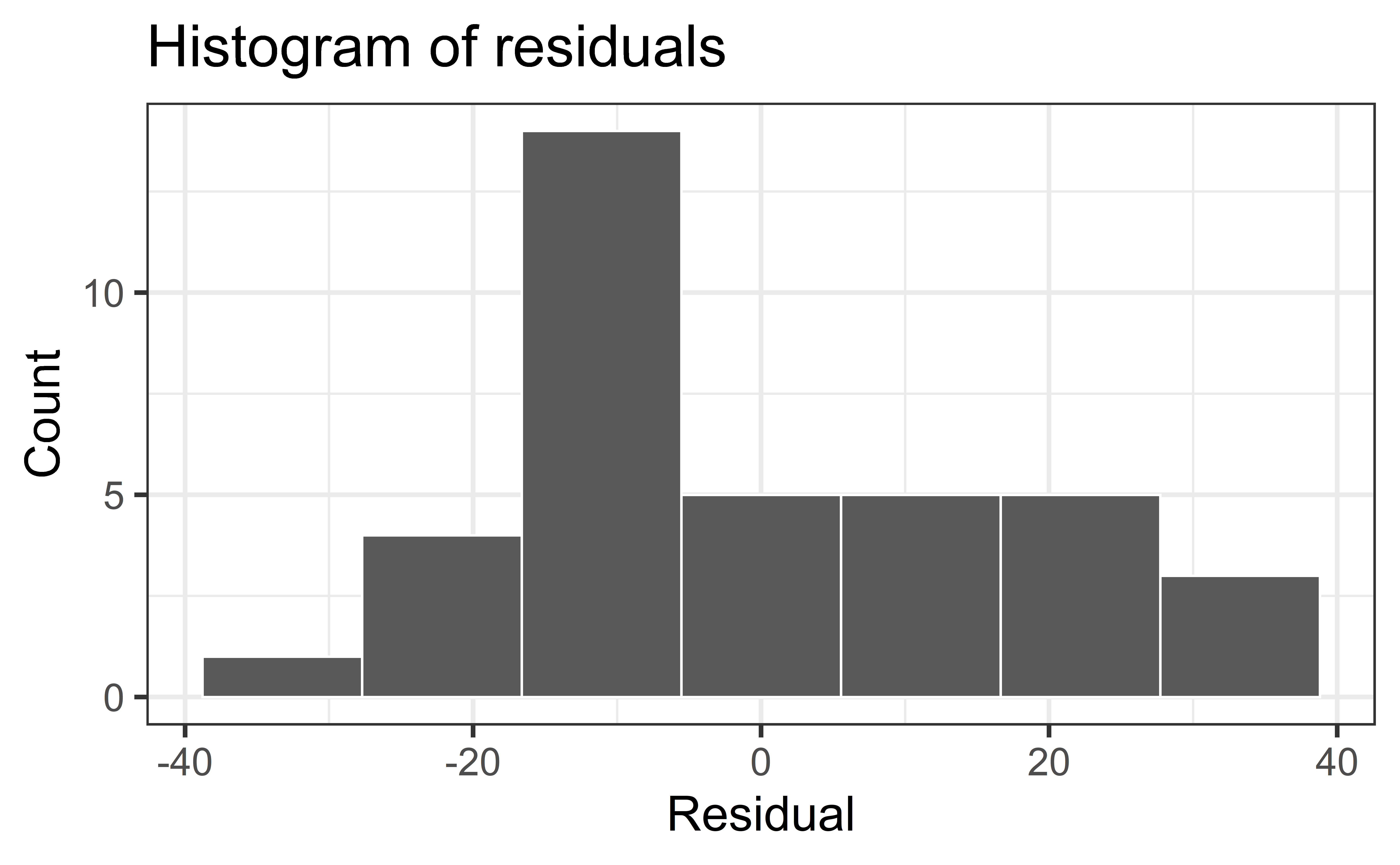
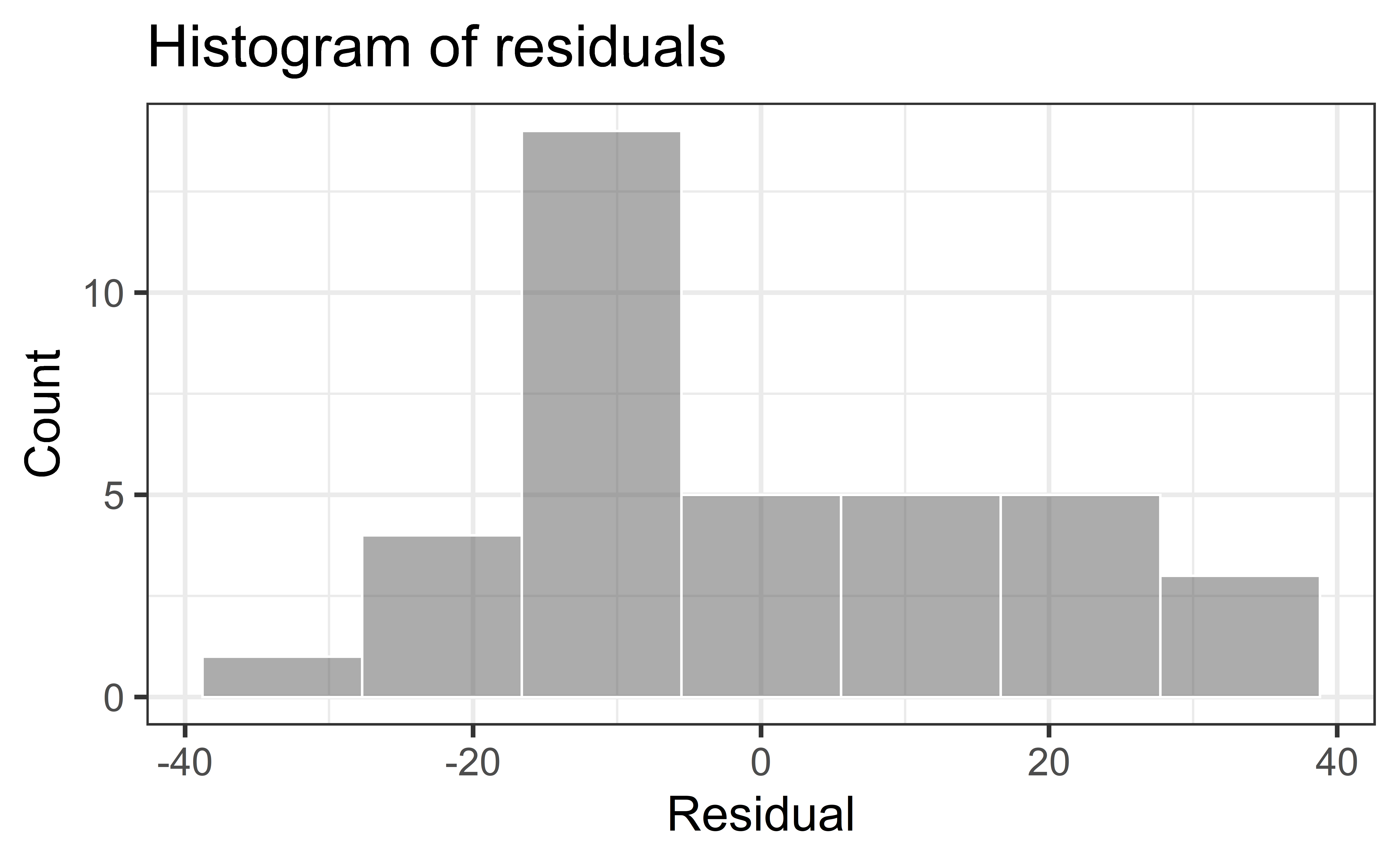
Normality

The linear model assumes that the distribution of \(Y\) is Normal for every value of \(X\)
This is impossible to check in practice, so we will look at the overall distribution of the residuals to assess if the normality assumption is satisfied
Normality satisfied if a histogram of the residuals is approximately normal
- Can also check that the points on a normal QQ-plot falls along a diagonal line
Most inferential methods for regression are robust to some departures from normality, so we can proceed with inference if the sample size is sufficiently large, \(n > 30\)

Normality

Check normality using a QQ-plot

Code

gf_histogram(~.resid, data = heb_aug,
             bins=7, color = "white") |> 
  gf_labs(
    x = "Residual",
    y = "Count",
    title = "Histogram of residuals"
  )

Code

gf_qq(~.resid, data = heb_aug) |> 
  gf_qqline() |>  
  gf_labs(x = "Theoretical quantile", 
       y = "Observed quantile", 
       title = "Normal QQ-plot of residuals")

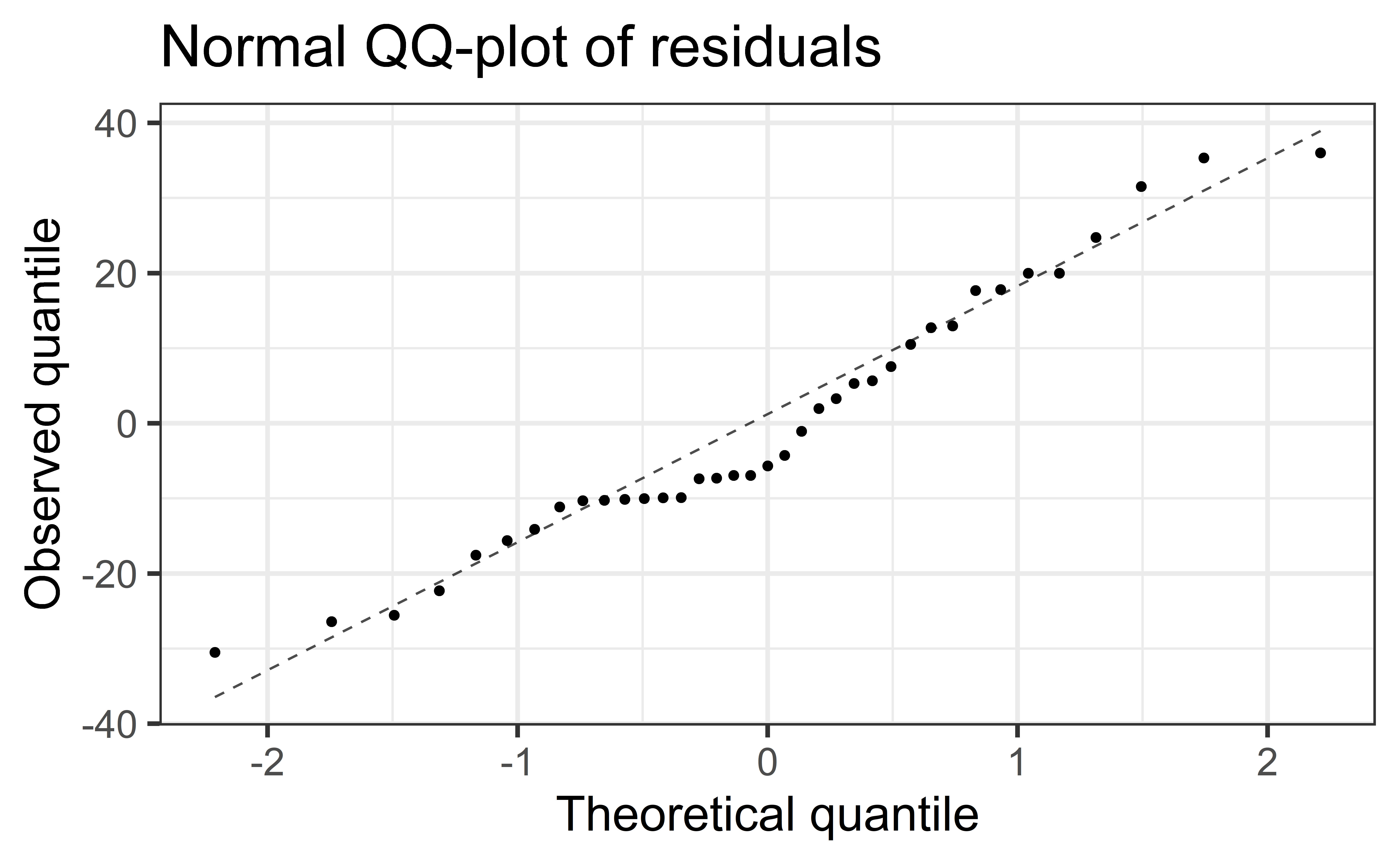
Assess whether residuals lie along the diagonal line of the Quantile-quantile plot (QQ-plot).
If so, the residuals are normally distributed.

Normality

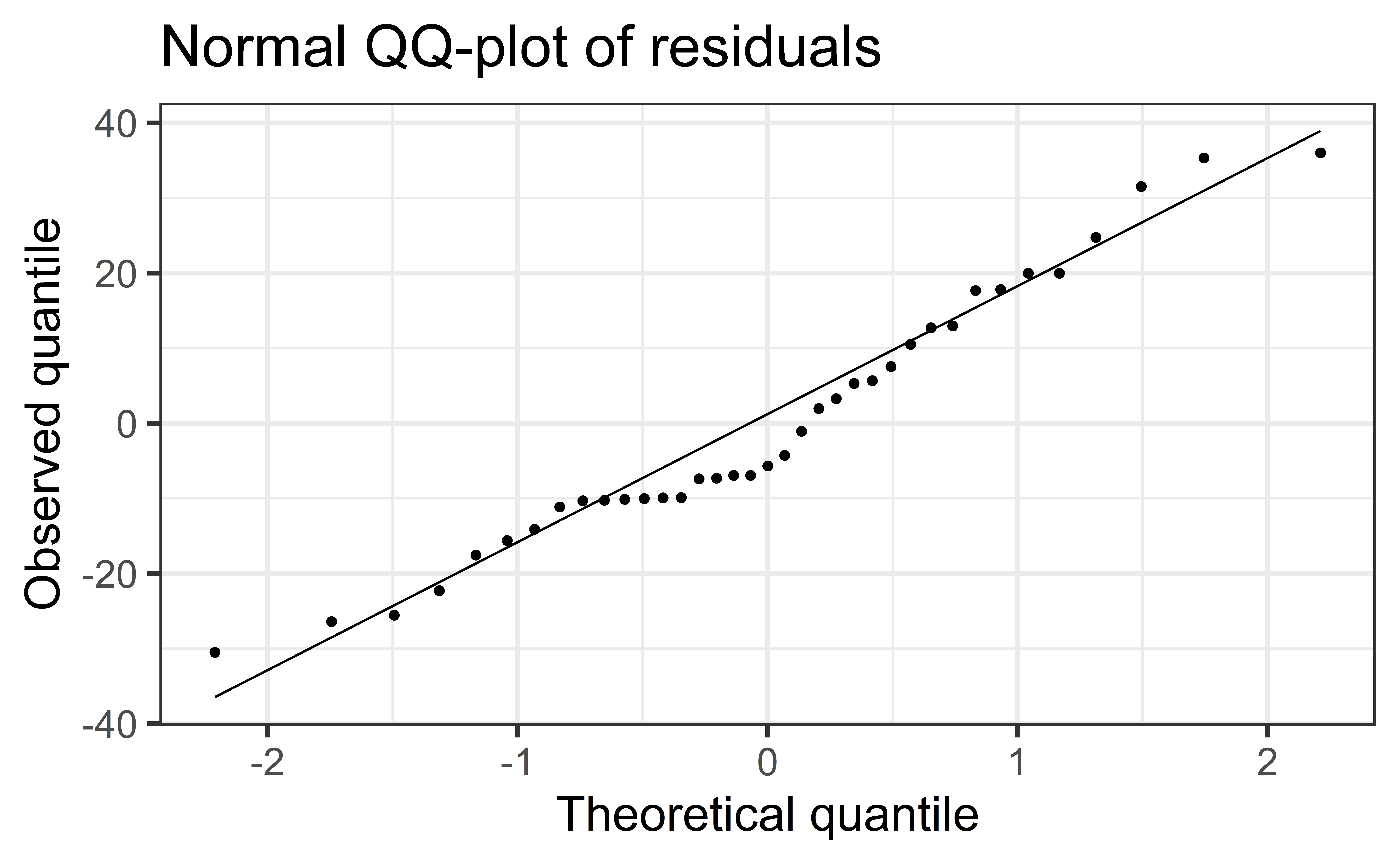
❌ The residuals do not appear to follow a normal distribution, because the points do not lie on the diagonal line, so normality is not satisfied.

✅ The sample size \(n = 37 > 30\), so the sample size is large enough to relax this condition and proceed with inference.

Independence

We can often check the independence assumption based on the context of the data and how the observations were collected
Two common violations of the independence assumption:
- Serial Effect: If the data were collected over time, plot the residuals in time order to see if there is a pattern (serial correlation)
- Cluster Effect: If there are subgroups represented in the data that are not accounted for in the model (e.g., type of supermarket), you can color the points in the residual plots by group to see if the model systematically over or under predicts for a particular subgroup

Independence

Recall the description of the data:

Average household income (per zip code) and number of organic vegetable offerings in San Antonio, TX
Data from HEB website, compiled by high school student Linda Saucedo, Fall 2019

❌ Based on the information we have, it’s unclear if the data are independent. In fact, I’d guess that they are likely geographically correlated.

Recap

Used residual plots to check conditions for SLR:

Linearity
Constant variance

Normality
Independence

Which of these conditions are required for fitting a SLR (and not doing any inference)?
Which for simulation-based inference for the slope for an SLR?
Which for inference with mathematical models?

03:00