SLR: Simulation-based inference
Bootstrap confidence intervals for the slope
AE 02 Follow-up
AE 02 Follow-up
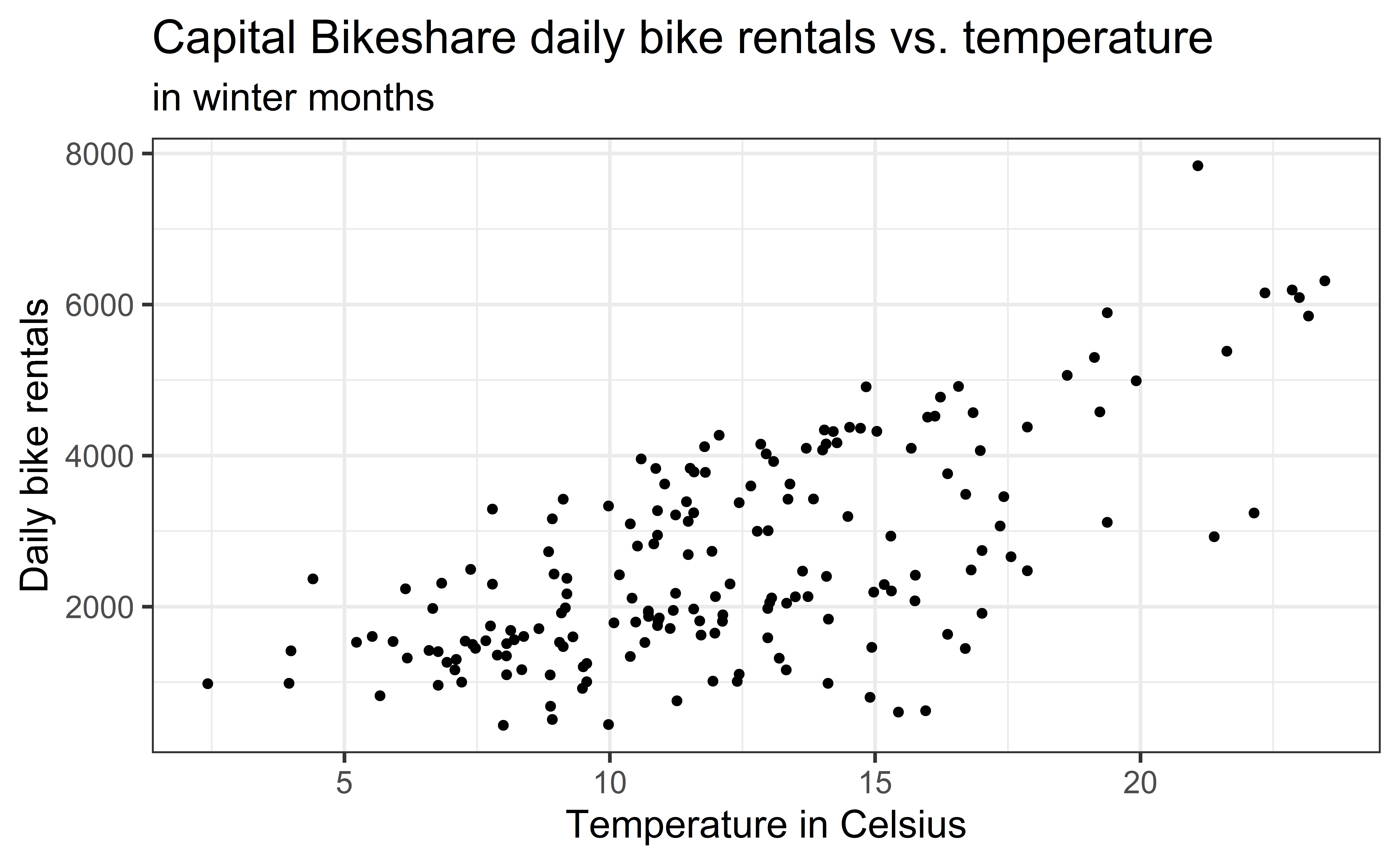
Goal: Use simple linear regression to model the relationship between temperature and daily bike rentals in the winter season
AE 02 Follow-up
Statistical Model:
\[count = \beta_0 +\beta_1 ~ temp\_orig + \epsilon, \hspace{5mm} \epsilon \sim N(0, \sigma_{\epsilon}^2)\]
. . .
winter_fit <- lm(count ~ temp_orig, data = winter)

tidy(winter_fit) |> kable(digits = 3)| term | estimate | std.error | statistic | p.value |
|---|---|---|---|---|
| (Intercept) | -111.038 | 238.312 | -0.466 | 0.642 |
| temp_orig | 222.416 | 18.459 | 12.049 | 0.000 |
AE 02 Follow-up
Use the output to write out the estimated regression equation.
\[ \hat{count} = -111.038 + 222.416 ~temp\_orig \]
LaTex:
\$\$\hat{count} = -111.038 + 222.416 ~ temp\_orig\$\$
Your turn!
Interpret the slope in the context of the data.
Why is there no error term in the regression equation?
Simulation-based inference
Bootstrap confidence intervals
Topics
- Find range of plausible values for the slope using bootstrap confidence intervals
Computational setup
# load packages
library(tidyverse)   # for data wrangling and visualization
library(ggformula)  # for modeling
library(scales)      # for pretty axis labels
library(knitr)       # for neatly formatted tables
library(kableExtra)  # also for neatly formatted tablesf


# set default theme and larger font size for ggplot2
ggplot2::theme_set(ggplot2::theme_bw(base_size = 16))
Data: San Antonio Income & Organic Food Access
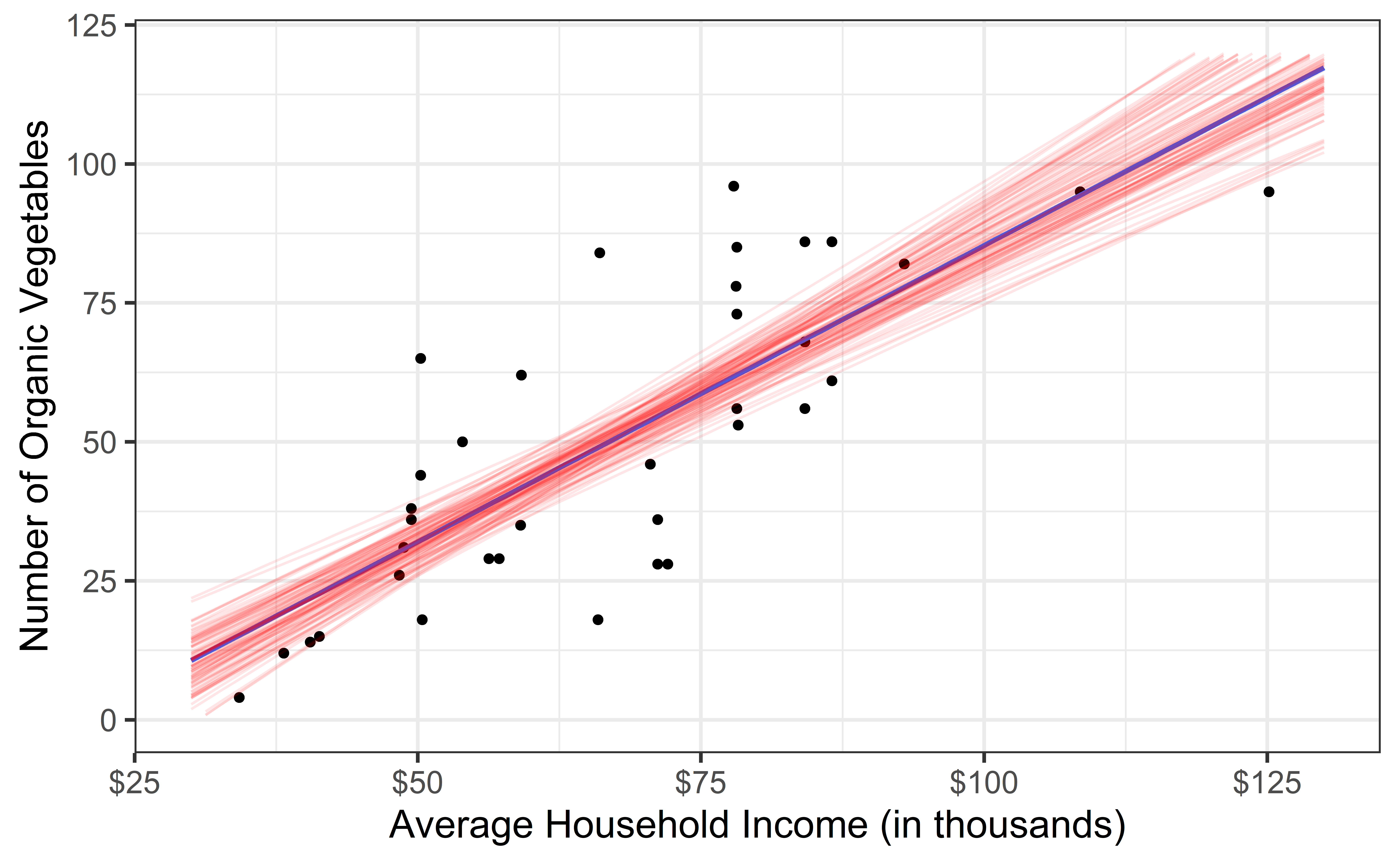
- Average household income (per zip code) and number of organic vegetable offerings in San Antonio, TX
- Data from HEB website, compiles by high school student Linda Saucedo, Fall 2019
- Source: Skew The Script
![]()
Goal: Use the average household income to understand variation in access to organic foods.
Exploratory data analysis
Code
heb <- read_csv("data/HEBIncome.csv") |>
  mutate(Avg_Income_K = Avg_Household_Income/1000)

gf_point(Number_Organic ~ Avg_Income_K, data = heb, alpha = 0.7) |>
  gf_labs(
    x = "Average Household Income (in thousands)",
    y = "Number of Organic Vegetables",
  ) |>
  gf_refine(scale_x_continuous(labels = label_dollar()))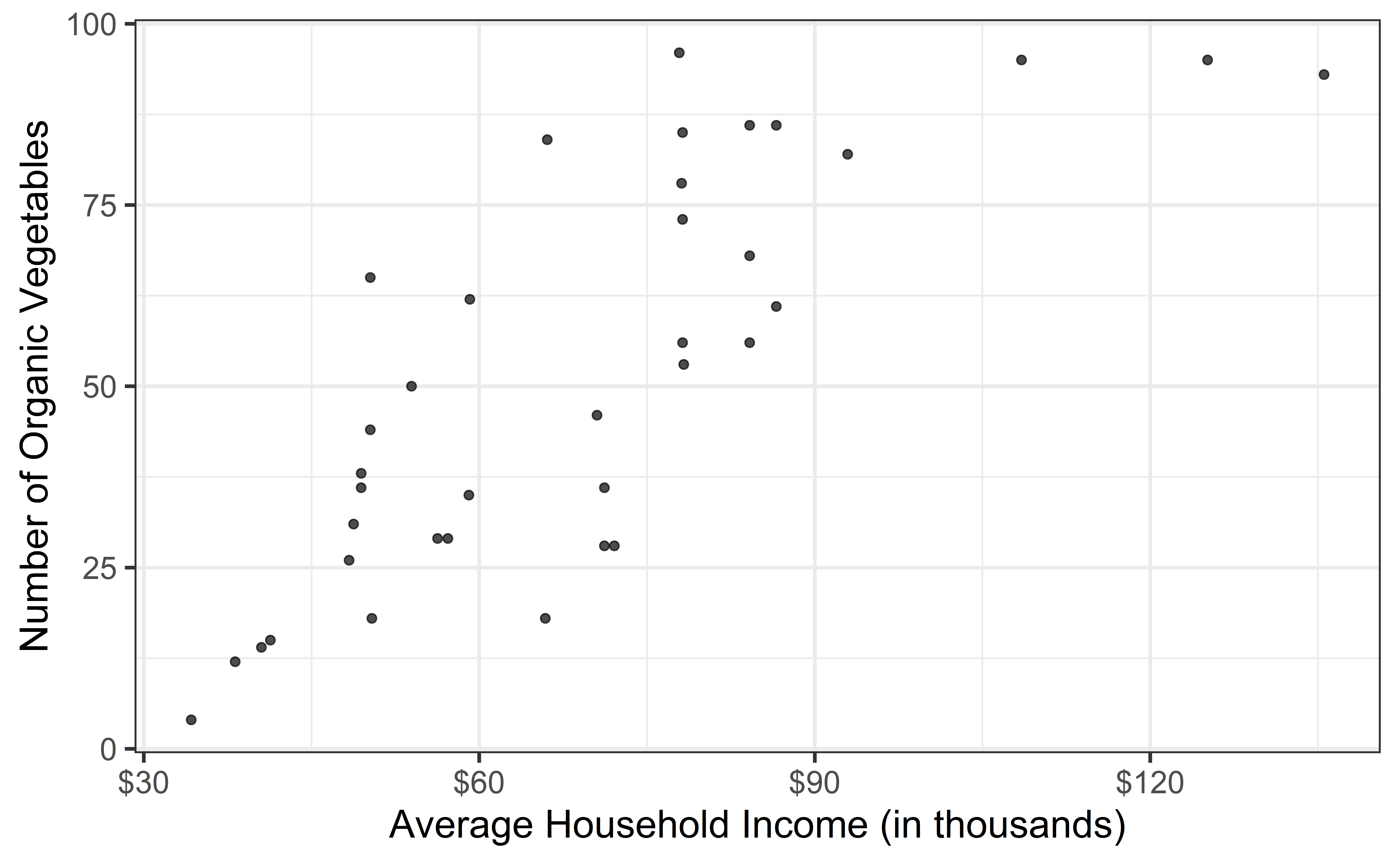
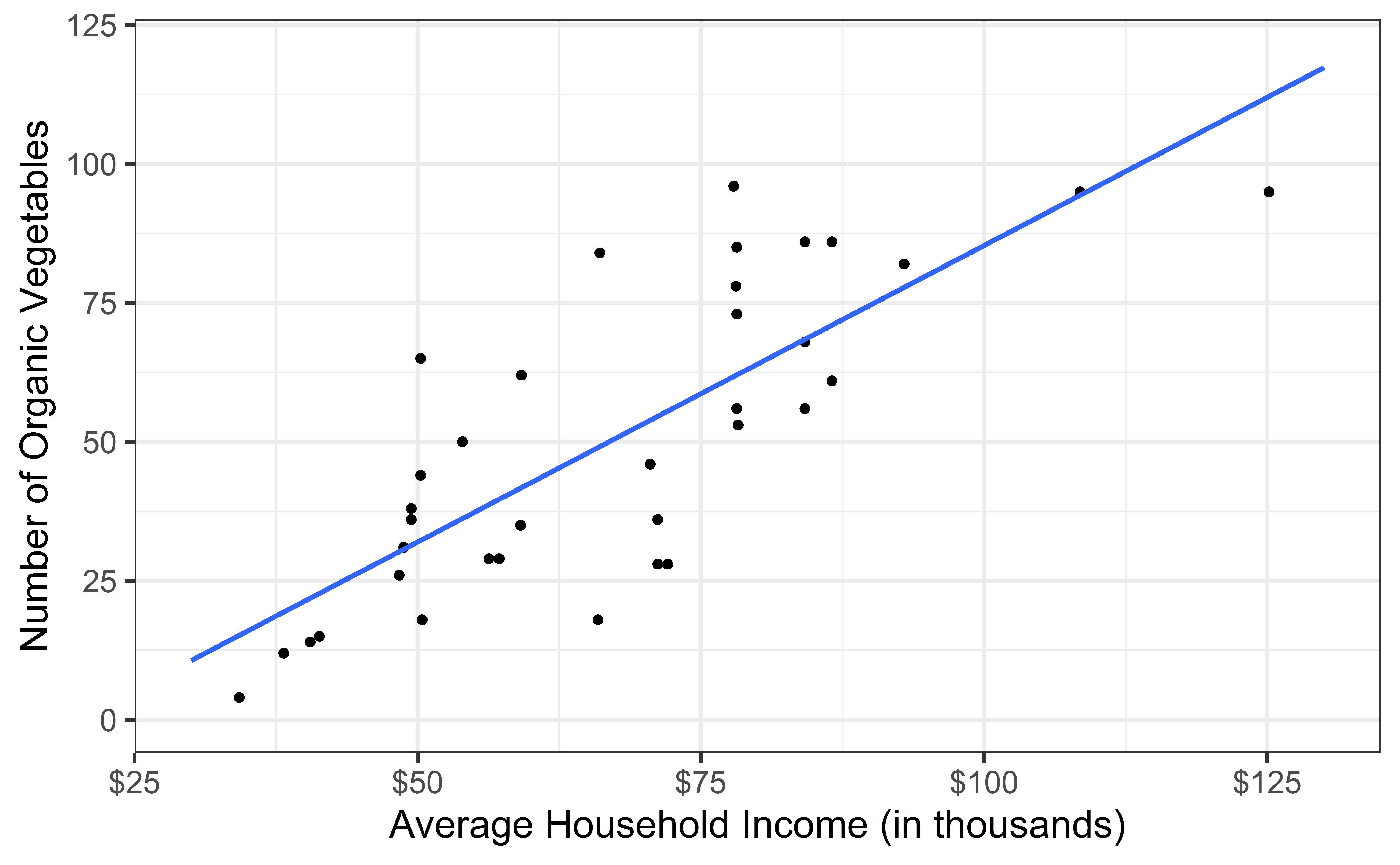
Modeling
heb_fit <- lm(Number_Organic ~ Avg_Income_K, data = heb)

tidy(heb_fit) |>
kable(digits=2) #neatly format table to 2 digits| term | estimate | std.error | statistic | p.value |
|---|---|---|---|---|
| (Intercept) | -14.72 | 9.30 | -1.58 | 0.12 |
| Avg_Income_K | 0.96 | 0.13 | 7.50 | 0.00 |
. . .
- Intercept: HEBs in Zip Codes with an average household income of $0 are expected to have -14.72 organic vegetable options, on average.
- Is this interpretation useful?
- Slope: For each additional $1,000 in average household income, we expect the number of organic options available at nearby HEBs to increase by 0.96, on average.
From sample to population
For each additional $1,000 in average household income, we expect the number of organic options available at nearby HEBs to increase by 0.96, on average.
- Estimate is valid for the single sample of 37 HEBs
- What if we’re not interested quantifying the relationship between the size and price of a house in this single sample?
- What if we want to say something about the relationship between these variables for all supermarkets in America?
Statistical inference
Statistical inference refers to ideas, methods, and tools for to generalizing the single observed sample to make statements (inferences) about the population it comes from
For our inferences to be valid, the sample should be random and representative of the population we’re interested in
Inference for simple linear regression
Calculate a confidence interval for the slope, \(\beta_1\)
Conduct a hypothesis test for the slope, \(\beta_1\)
Why not \(\beta_0\)?
We can but it isn’t super interesting typically
. . .
What is a confidence interval?
What is a hypothesis test?
Confidence interval for the slope
Confidence interval
- Confidence interval: plausible range of values for a population parameter
- single point estimate \(\implies\) fishing in a murky lake with a spear
- confidence interval \(\implies\) fishing with a net
- We can throw a spear where we saw a fish but we will probably miss, if we toss a net in that area, we have a good chance of catching the fish
- If we report a point estimate, we probably will not hit the exact population parameter, but if we report a range of plausible values we have a good shot at capturing the parameter
- High confidence \(\implies\) wider interval (larger net)
- Remember: single CI \(\implies\) either you hit parameter or you don’t
Confidence interval for the slope
A confidence interval will allow us to make a statement like “For each $1K in average income, the model predicts the number of organic vegetables available at local supermarkets to be higher, on average, by 0.96, plus or minus X options.”
. . .
Should X be 1? 2? 3?
If we were to take another sample of 37 would we expect the slope calculated based on that sample to be exactly 0.96? Off by 1? 2? 3?
The answer depends on how variable (from one sample to another sample) the sample statistic (the slope) is
We need a way to quantify the variability of the sample statistic
Quantify the variability of the slope
for estimation
- Two approaches:
- Via simulation (what we’ll do today)
- Via mathematical models (what we’ll do in the soon)
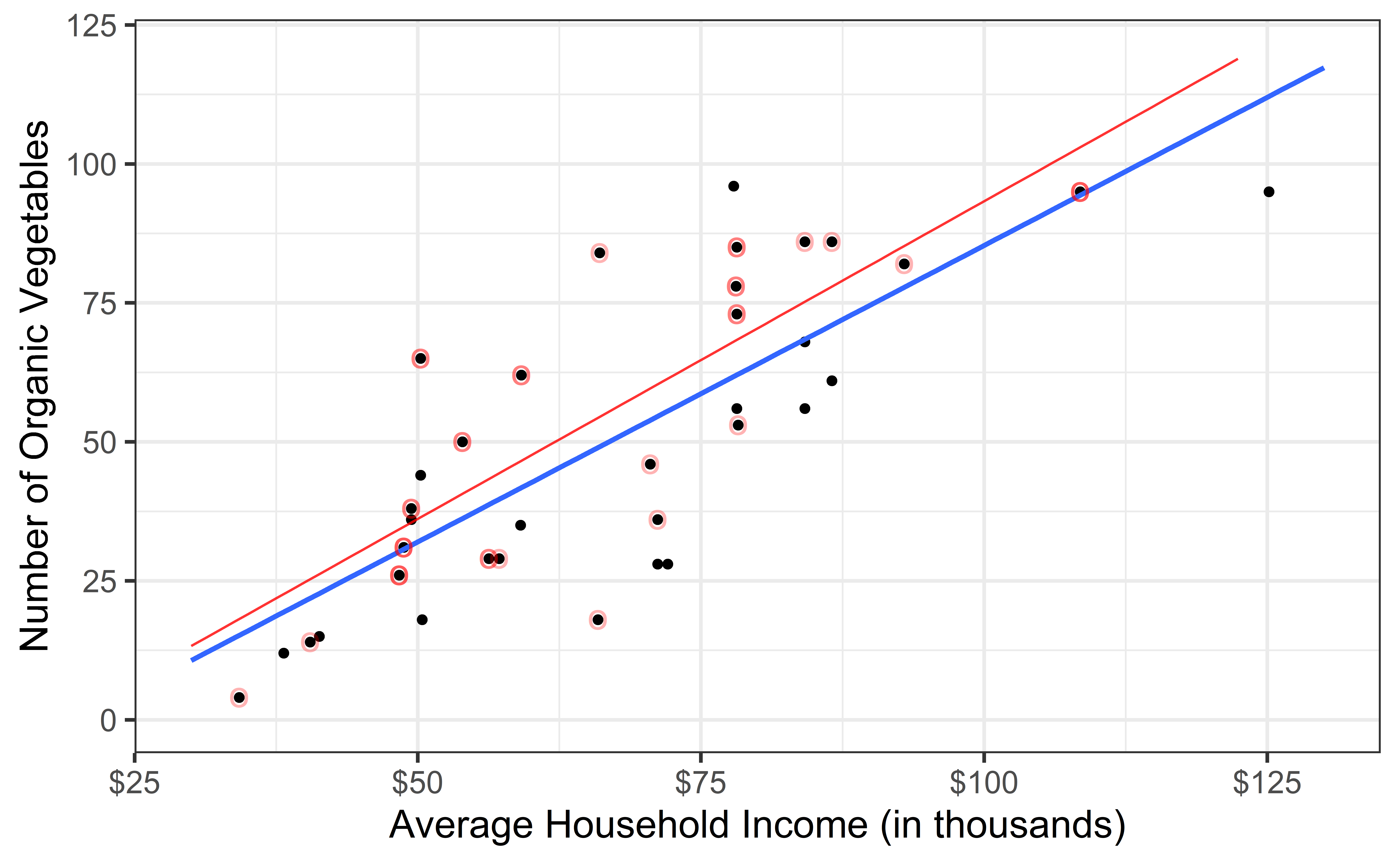
- Bootstrapping to quantify the variability of the slope for the purpose of estimation:
- Generate new samples by sampling with replacement from the original sample
- Fit models to each of the new samples and estimate the slope
- Use features of the distribution of the bootstrapped slopes to construct a confidence interval
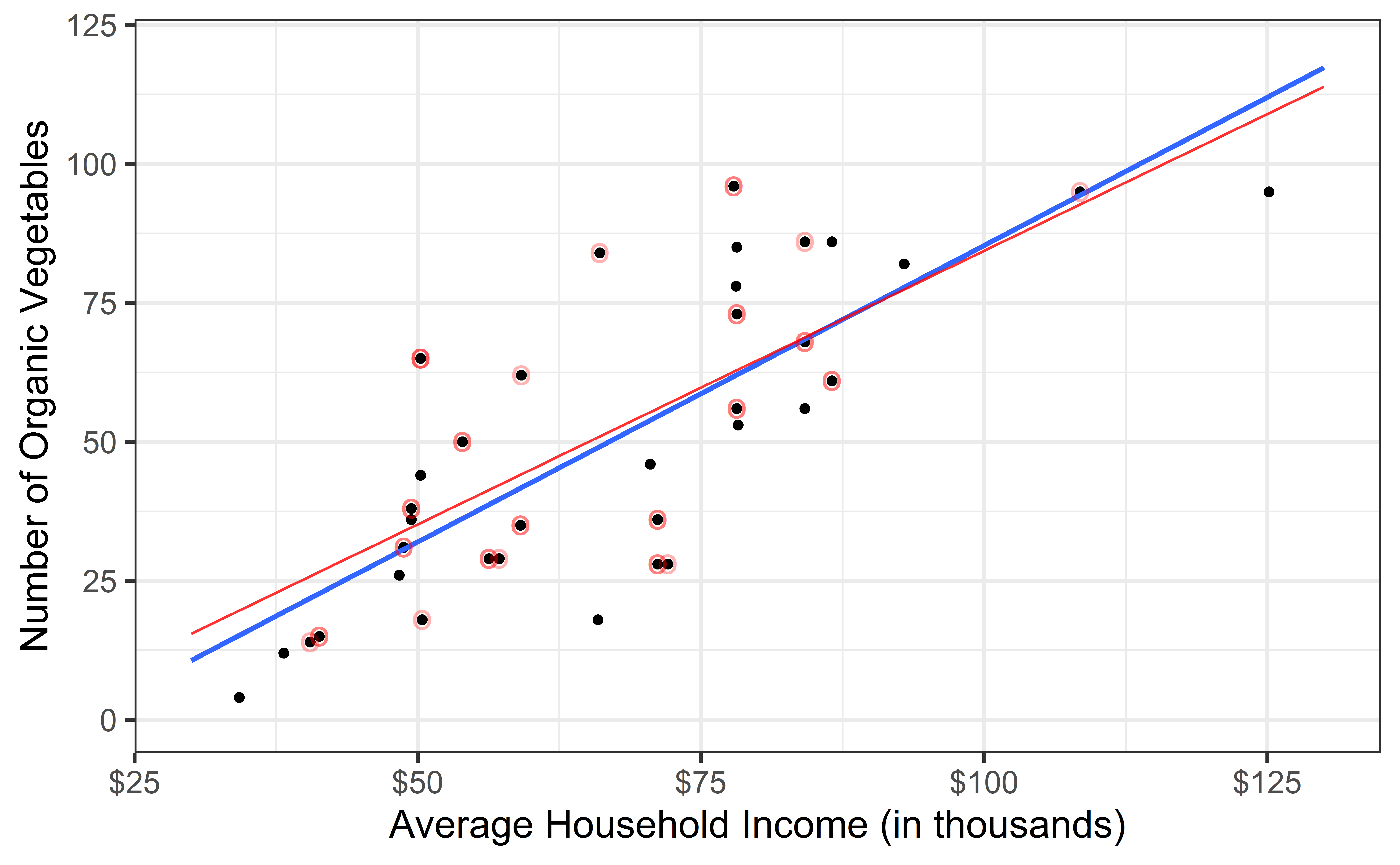
Original Sample
Bootstrap sample 1

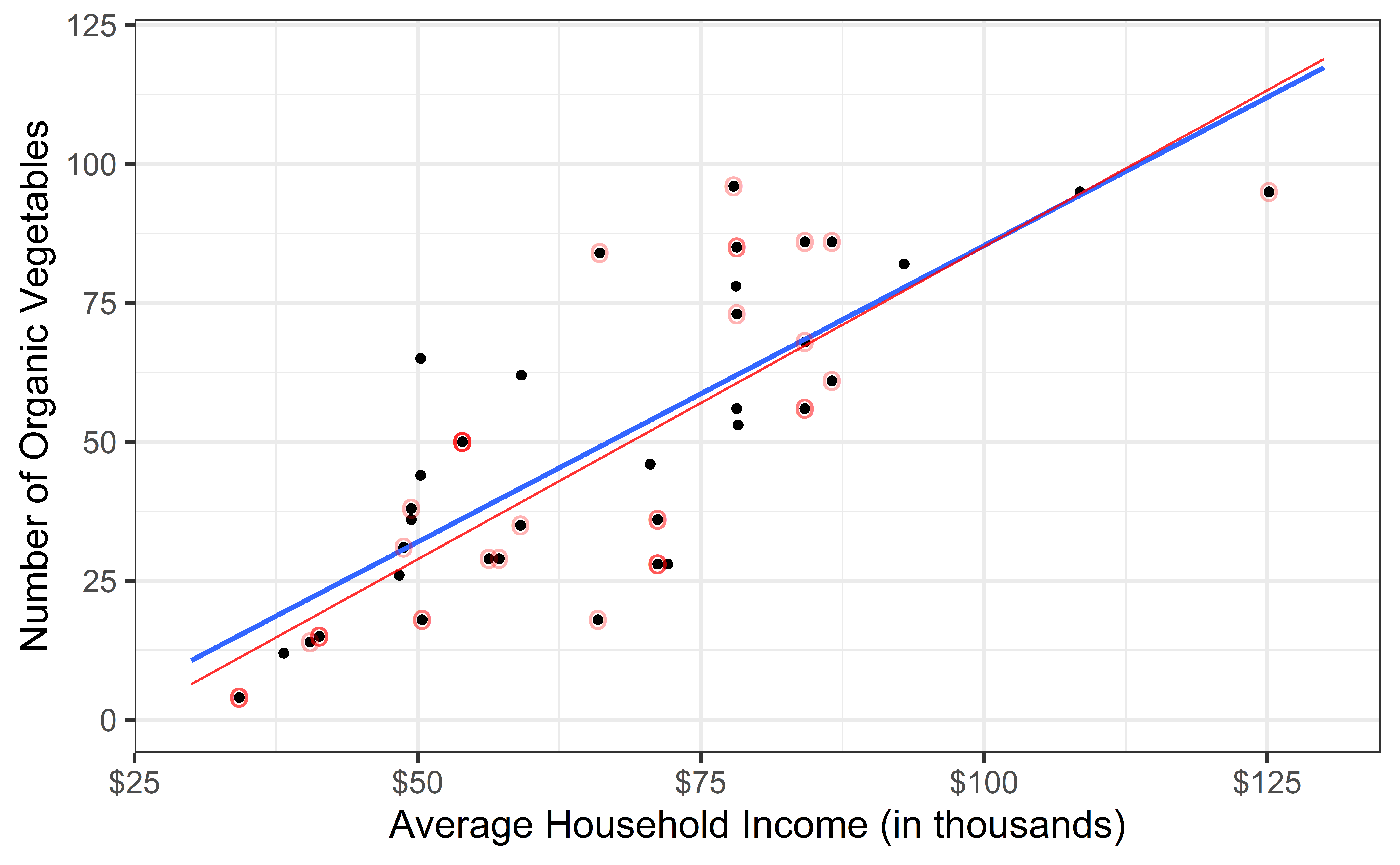
Bootstrap sample 2
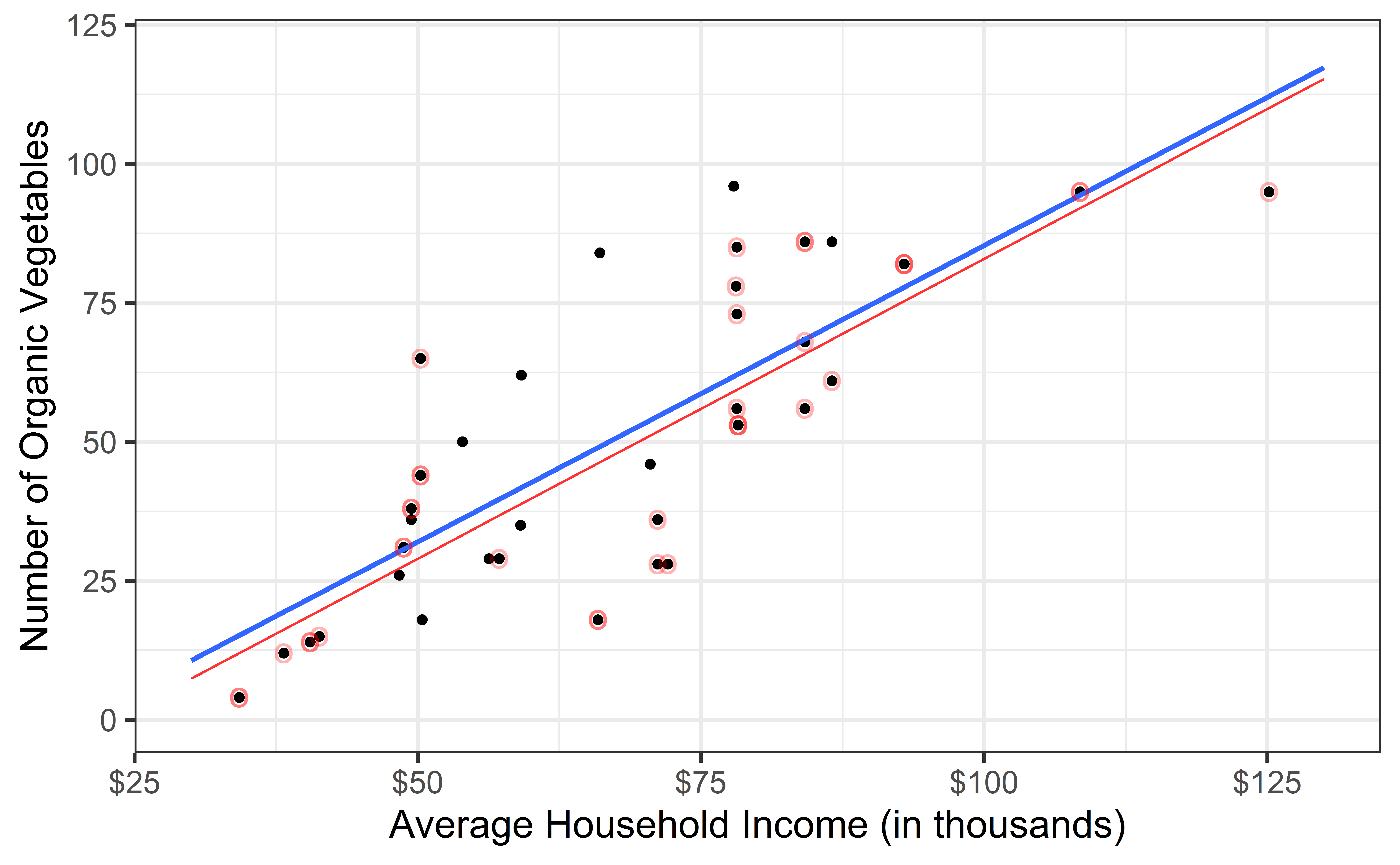
Bootstrap sample 3
Bootstrap sample 4
Bootstrap sample 5
Bootstrap samples 1 - 5
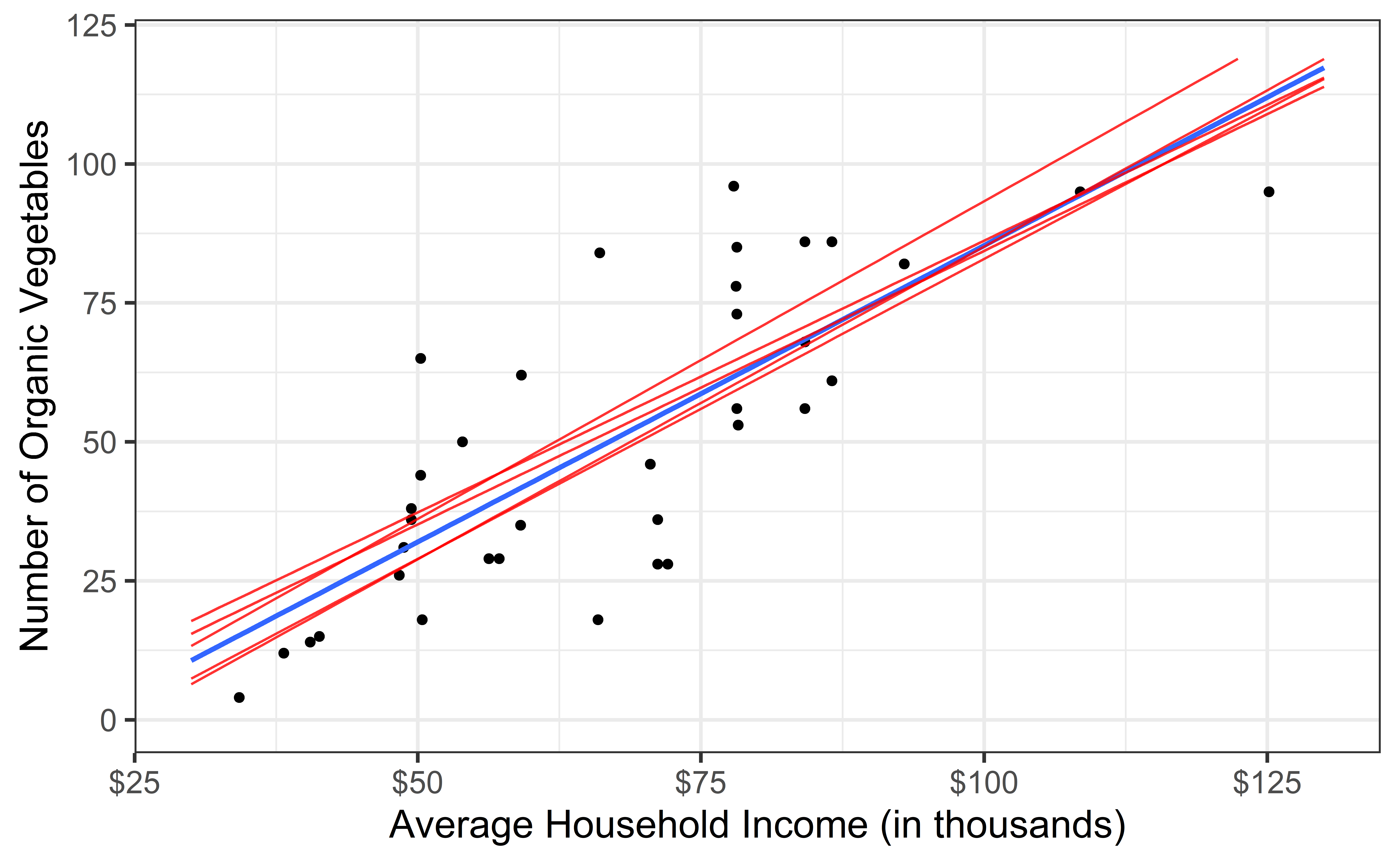
Bootstrap samples 1 - 100

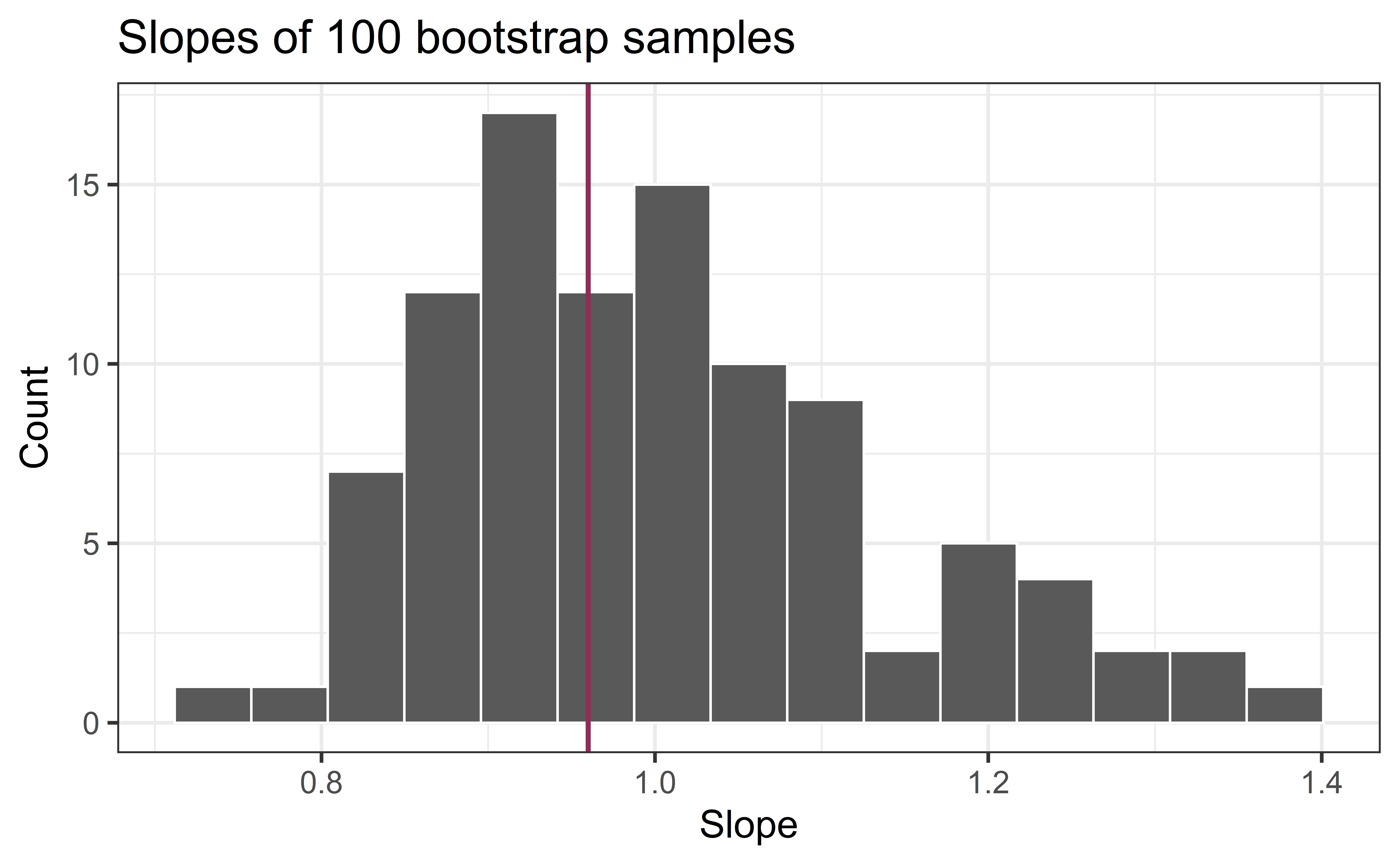
Slopes of bootstrap samples
Fill in the blank: For each additional $1k in average household income, the model predicts the number of organic vegetables available to be higher, on average, by 0.96, plus or minus ___.
Slopes of bootstrap samples
Fill in the blank: For each additional $1k in average household income, the model predicts the number of organic vegetables available to be higher, on average, by 0.96, plus or minus ___.

Confidence level
How confident are you that the true slope is between 0.8 and 1.2? How about 0.9 and 1.0? How about 1.0 and 1.4?
95% confidence interval
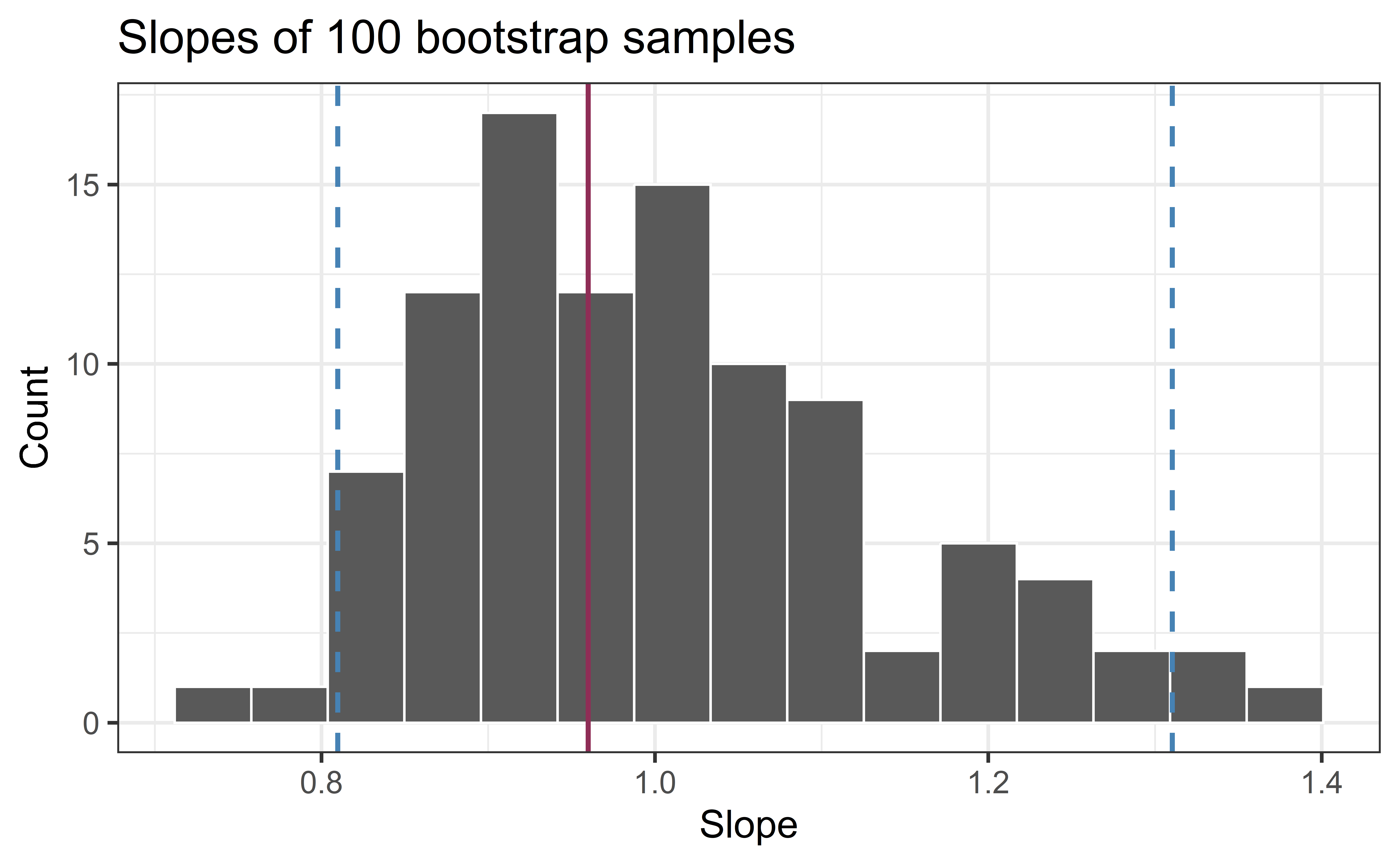
- 95% bootstrapped confidence interval: bounded by the middle 95% of the bootstrap distribution
- We are 95% confident that for each additional $1K in average household income, the model predicts the number of organic vegetables options at local supermarkets to be higher, on average, by 0.81 to 1.31.
Computing the CI for the slope I
Calculate the observed slope:
library(infer) # package that does Simulation-Based Inference

observed_fit <- heb |>
  specify(Number_Organic ~ Avg_Income_K) |>
  fit()

observed_fit
# A tibble: 2 × 2
term estimate
<chr> <dbl>
1 intercept -14.7
2 Avg_Income_K 0.959Computing the CI for the slope II
Take 100 bootstrap samples and fit models to each one:
set.seed(1120)

boot_fits <- heb |>
  specify(Number_Organic ~ Avg_Income_K) |>
  generate(reps = 100, type = "bootstrap") |>
  fit()

boot_fits
# A tibble: 200 × 3
# Groups: replicate [100]
replicate term estimate
<int> <chr> <dbl>
1 1 intercept -40.9
2 1 Avg_Income_K 1.25
3 2 intercept -23.9
4 2 Avg_Income_K 1.09
5 3 intercept -18.6
6 3 Avg_Income_K 1.02
7 4 intercept -1.96
8 4 Avg_Income_K 0.828
9 5 intercept -15.1
10 5 Avg_Income_K 0.951
# ℹ 190 more rowsComputing the CI for the slope III
Percentile method: Compute the 95% CI as the middle 95% of the bootstrap distribution:
Precision vs. accuracy
If we want to be very certain that we capture the population parameter, should we use a wider or a narrower interval? What drawbacks are associated with using a wider interval?
. . .

Precision vs. accuracy
How can we get best of both worlds – high precision and high accuracy?
Changing confidence level
How would you modify the following code to calculate a 90% confidence interval? How would you modify it for a 99% confidence interval?
Changing confidence level
## confidence level: 90%
get_confidence_interval(
  boot_fits, point_estimate = observed_fit,
  level = 0.90, type = "percentile"
)
# A tibble: 2 × 3
term lower_ci upper_ci
<chr> <dbl> <dbl>
1 Avg_Income_K 0.829 1.23
2 intercept -31.7 -3.76## confidence level: 99%
get_confidence_interval(
boot_fits, point_estimate = observed_fit,
level = 0.99, type = "percentile"
)# A tibble: 2 × 3
term lower_ci upper_ci
<chr> <dbl> <dbl>
1 Avg_Income_K 0.795 1.36
2 intercept -43.3 -0.535Application exercise
Recap
Population: Complete set of observations of whatever we are studying, e.g., people, tweets, photographs, etc. (population size = \(N\))
Sample: Subset of the population, ideally random and representative (sample size = \(n\))
Sample statistic \(\ne\) population parameter, but if the sample is good, it can be a good estimate
Statistical inference: Discipline that concerns itself with the development of procedures, methods, and theorems that allow us to extract meaning and information from data that has been generated by stochastic (random) process
We report the estimate with a confidence interval, and the width of this interval depends on the variability of sample statistics from different samples from the population
Since we can’t continue sampling from the population, we bootstrap from the one sample we have to estimate sampling variability